Fluorescence Decay Panel

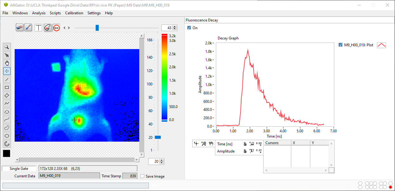
The Fluorescence Decay panel can be displayed using the pull-down list at the top-right of the main AlliGator window.

In the example shown below, a point ROI was selected in the Tool Palette on the lefthand side of the Source Image, and a ROI decay analysis performed using the Analysis:Current ROI Analysis menu item (Ctrl+A). While a Single Gate image is shown in the Source Image, the analysis encompasses all gate images, whose intensities at that selected pixels are represented as a decay curve (named M9_H00_019: Plot [1]).

The Decay Graph is a feature-rich object which is comprised of different parts, some of which are common to all graph objects and are described in the Graph Object Anatomy page.

In particular, different types of contextual menus are accessible, depending on which area of the graph the user right-clicks:

• Plot Menu

• Decay Graph Custom Menu

• Cursor Legend Menu

The first and last ones are similar for all graph objects and are described in detail in the Graph Object Anatomy page.

An overview of the Decay Graph custom menu is presented below, specific functionalities being described in other pages of the manual (linked to in the section below).

Decay Graph Custom Menu

All items not highlighted in the image below are standard graph object contextual menu items and are described in the Graph Object Anatomy page (Custom Graph Menu section).

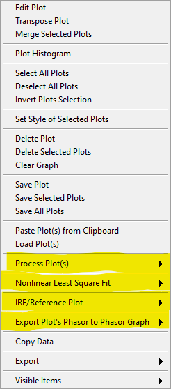
This section will briefly discuss the highlighted submenus, whose functions are described in specific pages.

Process Plot(s)

This menu, shown below, allows various types of plot transformations to be performed. The highlighted operations are also available as pre-processing operations applied to each decay (before plotting in the Decay Graph, or other computations involving decays such as phasor calculation) and are discussed in the Decay Preprocessing page.

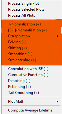
• Process Single Plot: This option does not do anything on a plot, but is used to instruct AlliGator to operate on a single plot. The checkmark in front of it indicates that this is the current mode of operation for all the functions in the menu followed by the (+) suffix.

• Process Selected Plot: This option does not do anything on any plot, but is used to instruct AlliGator to operate on all selected plots. The checkmark in front of it indicates that this is the current mode of operation for all the functions in the menu followed by the (+) suffix.

• Process All Plots: This option does not do anything on any plot, but is used to instruct AlliGator to operate on all plots. The checkmark in front of it indicates that this is the current mode of operation for all the functions in the menu followed by the (+) suffix.

• 1-Normalization: applies the 1-Normalization operation discussed in the Decay Preprocessing page.

• [0-1]-Normaliztion: applies the [0-1]-Normalization operation discussed in the Decay Preprocessing page.

• Extrapolation:Extrapolate Plot: extrapolates the selected plot(s) as discussed in the Decay Preprocessing page.

• Folding: folds the selected plot(s) as discussed in the Decay Preprocessing page.

• Shifting: shifts the selected plot(s) as discussed in the Decay Preprocessing page.

• Smoothing: smoothes the selected plot(s) using cubic splines as discussed in the Decay Preprocessing page.

• Straightening: straightens the selected plot(s) as discussed in the Decay Preprocessing page.

• Convolution with IRF: convolves the selected plot(s) with the stored reference decay.

• Cumulative Function: computes the cumulative function of the selected plot(s).

• Denoising: processes the selected plot(s) with the Wavelet Analysis Denoise algorithm (see https://www.ni.com/docs/en-US/bundle/labview-advanced-signal-processing-toolkit-api-ref/page/lvwavelettk/wa_de_noise.html for details) using the Wavelength Analysis Options defined in the Settings:Fluorescence Decay:Advanced Analysis panel.

• Rebinning: changes the bin size of the selected plot(s). A dialog window opens up to define the new (larger) bin size.

• Tail Smoothing: smoothes the tail (part of the decay past the maximum) of the selected plot(s) using cubic splines as described above.

Plot Math

This sub-menu comprises the following functions:

• y -> f(y) Transform: selecting this item opens up a dialog window to enter an algebraic formula: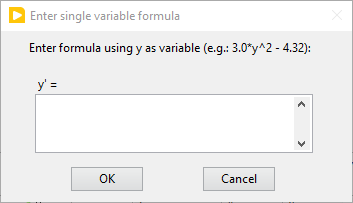

  

  The corresponding amplitude values of the plot (y) will be modified and replaced by y’ as defined by the formula (assuming that the syntax is correct. For a list of supported functions, please refer to this LabVIEW help page).

• (x, y) >> (f, g)(x, y) Transform: selecting this item opens up a dialog window to enter an algebraic formula: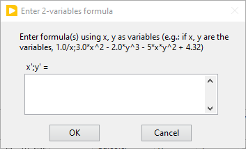

  

  The corresponding time (x) and amplitude (y) values of the plot will be modified and replaced by (x’, y’) as defined by the formulas (assuming that the syntax is correct. For a list of supported functions, please refer to this LabVIEW help page).

• Two-Plot Algebra: selecting this item opens up a dialog window to enter an algebraic formula: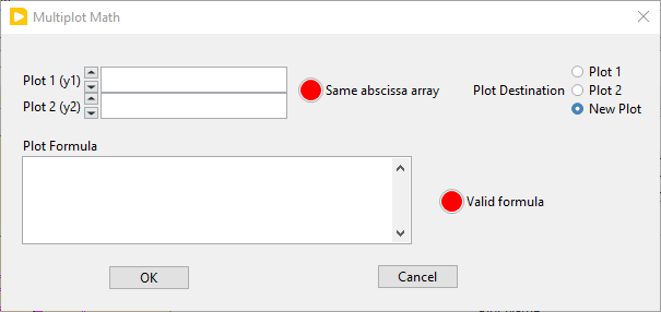

  

  The two plots to be processed can be selected in the Plot 1 and Plot 2 pull-down lists. Only plots with identical abscissa (time axis) can be processed. The Same abcissa array LED turns green when this is the case.

  The first plot is referred to as y1 and the second plot as y2 in the Plot Formula box below, in which the desired formula can be entered.

  Example of valid Plot formula (where y1 represents the value of plot 1 at a given abscissa and y2 the value of the second plot at the same abscissa):

  2*y1 - 3*y2/((1.5e(-3))+y2)

  he list of supported functions can be found at https://www.ni.com/docs/en-US/bundle/labview/page/lvhowto/formula_node_and_express.html

  The list of supported operators can be found at: https://www.ni.com/docs/en-US/bundle/labview/page/lvhowto/precedence_of_operators_in.html

  Note that the exponentiation operator is ‘**’, i.e. the square of y is noted y**2.

• Average Selected Plots: This function does what it says and creates an additional plot.

• Compute Average Lifetime: computes the average lifetime of the selected decay using Average Lifetime Options defined in the Fluorescence Decay:Advanced Analysis panel of the Settings window.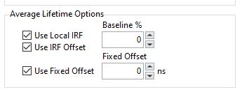

  

Nonlinear Least Square Fit

This menu currently contains a single item, whose functionality is described in the Decay Fitting page.

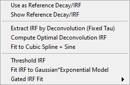
IRF/Reference Plot

This menu allows defining the reference decay used either for temporal shifting (see Decay Shifting in the Decay (Pre-)Processing page of the manual) or reconvolution of fit models when using the NLSF analysis features of AlliGator. More details on the functions of this menu can be found in the Decay Fitting page.

Export Decay to Phasor Graph

This menu allows computing the phasor of a pre-computed decay and export the resulting phasor to the Phasor Graph. This is for instance useful to export a computed or recorded IRF to the Phasor Graph in order to subsequently use it as a calibration phasor.

Python Plugins

Python plugins menu items and submenus will appear at the bottom of the Decay Graph contextual menu. Their names and content will depend on each installation, but typically will contain some examples or default functionalities.

Notes

[1]

When the user-selected ROI has a name (that is, when it has been stored in the Source Image ROI Manager Window), this name is appended to the image name, instead of the generic Plot suffix. A number is autimatically added to the decay name if the same ROI is used several times, or unnamed ROIs are used.