Lifetime & Other Parameters Panel
Introduction
This panel contains the Lifetime & Other Parameters graph which receives plots
from several Analysis main menu functions, Phasor Graph right-click menu
functions as well as plots sent by Decay Fit Parameters Map right-click menu
functions. The plots therefore may have different meaning and sizes.
To account for this diversity, the graph has two vertical axes. The left axis
(Lifetime (ns)) corresponds to lifetime (or in general time) values, while
the right axis (Other Parameters) is typically used to plot NLSF parameters.
The horizontal axis might take on a different name depending on context (for
instance Time (s) for a time series analysis, or Intensity when plotting
a Lifetime vs Intensity plot). Axes labels can be edited in the Scale Legend
box (between the Graph Palette and Cursor Legend in the figure below) and
have only a visual aid function.
Each plot can be associated to either one of the two vertical axes by
right-clicking on the plot icon in the graph legend and navigating down to the
Y Scale menu:
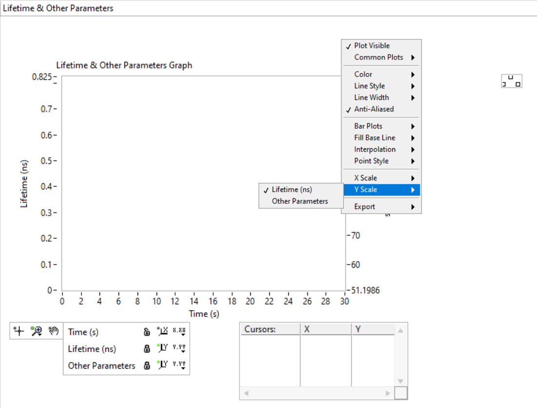
and selecting the relevant axis. Plots that “don’t look right” might just be associated with the wrong Y axis.
The following is a list of possible plots that will be sent to this panel.
Average lifetime
As discussed in the Phasor Ratio panel manual page, computation of a phasor ratio is generally accompanied by the calculation of the corresponding average lifetime, based on the formulas in the introduction to phasor ratio references in the Phasor Graph panel manual page.
Decay fit parameters
As discussed in the Fluorescence Decay Fitting manual page, it is possible to have the different parameters of a series of fits output sent as separate plots (one plot per selected parameter). These plots are sent to the Lifetime & Other Parameters graph.
Decay shifts
When decays are aligned with respect to a Reference Decay as part of a decay
preprocessing step, the corresponding computed temporal shifts are stored in
memory. The corresponding series of shifts can be represented as a plot using
the Plot Decay Shifts right-click menu item of the Lifetime & Other
Parameters graph.
Lifetime & Other Parameters graph context menu
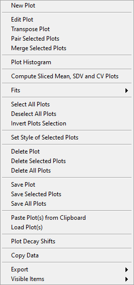
The Lifetime & Other Parameters graph has some specific context menu items described next:
.
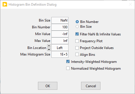
Transpose Plot: thePlot Histogrammenu item described later only works on the vertical coordinate. In order to histogram the horizontal coordinate of a scatterplot, it is therefore necessary to transpose that plot using this function.Pair Selected Plot: when two plots have the same abscissa array, they can be written \({(x_i, y_i)}_{i = 1,..,n}\) and \({(x_i, g_i)}_{i = 1,..,n}\). Pairing these two plots consists in building the following plot: \({(y_i, g_i)}_{i = 1,..,n}\).Merge Selected Plots: appends several plots to one another to form a larger plot containing all their data.Plot Histogram: builds an histogram of the selected plot (with user-defined options described next). This opens the Histogram window (described in the corresponding page of the manual, where a number of further analyses can be carried out. The histogram options dialog is shown below:
.
The histogram is defined by its Bin Number or Bin Size, depending on the radio button selection on the right. The corresponding parameter needs to be specified on the left.
Optionally, the Min Value and/or Max Value to be included in the analysis can be specified (by default, these parameters are set to -Inf and +Inf, meaning that all values are histogrammed).
Pathological values can be rejected before building the histogram (Filter NaN & Infinite Values option).
The histogram can be normalized to a sum of 1, making in a Frequency Plot if that option is selected.
The histogram can be represented Left-aligned, Centered or Right-aligned depending on the selected Bin Location option.
The bins can be “aligned” (Align Bins checkbox), that is, the bin boundaries are multiples of the Bin Size (either the entered one, or the calculated one).
The maximum number of bin can be limited to the Max Histogram Size to avoid cases where the Min and Max values and bin size result in a huge number of (mostly empty) bins, letting AlliGator run out of memory.
Values outside the Min and Max Values can be included in the first and last bin of the histogram if the Project Outside Values option is selected.
An option to compute Intensity-Weighted Histogram can be checked off to fill each bin with the associated pixel/ROI intensity value rather than 1.
In order to compare intensity-weighted histograms with unweighted ones, the option to compute a Normalized Weighted Histogram can be checked off. The corresponding histogram is normalized such that the sum of all its bins is equal to that of the unweighted histogram.
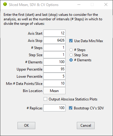
Compute Sliced Mean, SDV & CV Plots: this function allows computing the mean, standard deviation (SDV) and coefficient of variation (CV) of a plot by “slice”. Slices correspond to subsets of the plot’s data defined by fixed ranges of the abscissa values. The function requires input from the user, provided in the Sliced Mean, SDV & CV Options window:
.
The slices are defined by:
the first and last values of the abscissa considered (Axis Start and Axis Stop), which can be manually entered or automatically set to the data minimum and maximum values if the Use Data Min/Max checkbox is checked off.
the number of slices (# Steps), their “width” (Step Size) or their content (# Elements) depending on the radio button selection. The corresponding parameter to the left needs to be provided by the user.
within the data in each slice, the data Lower and Upper Percentile retained in the analysis (allowing to reject outliers). Enter 100 and 0 respectively to keep all data.
Min # Data Points/Slice: the minimum number of data points in a slice to compute the mean and SDV (a low number results in more statistical uncertainty).
the Bin Location (Left, Center, Mean, Right) defines each bin’s abscissa: either the bin’s lower bound, its center, the mean of all data in the bin or the bin’s upper bound.
If the Output Abscissa Statistics Plots checkbox is unchecked, the only plots created are the Mean, Standard Deviation and # Points plots as a function of the slice Start value. If the checkbox is checked off, two additional plots are output: the Mean and Standard Deviation of the abscissa values in the slice.
If the Bootstrap CV’s SDV checkbox is checked off, the # Replicas parameter is shown, which allows estimating the standard deviation of the CV of each slice by bootstrapping the sliced data. A reasonable number of replicas is the number of bin elements.
(last updated: 2024-09-09)