Fluorescence Decay Fitting

AlliGator offers basic capabilities to analyze data using standard techniques of fluorescence decay fitting:

• Individual decays can be fitted with a single or double-exponential decay model convolved with or without an experimental instrument response function (IRF).

• Multiple ROIs in the image source can be fitted, the resulting parameters being output as maps (see Decay Fit Parameter Map Panel)

• Series analysis of a ROI in the image source can be done one ROI at a time (the same ROI is used throughout the series), or a list of ROIs can be used, one dataset in the series using one of the ROI in the list (in the order they appear in the list). In both cases, selected parameters are output as individual plots (one plot per parameter, one point per dataset).

These different capabilities are described next.

Instrument Response Function (IRF)

As discussed in the IRF/Reference Plot section of the Fluorescence Decay Panel manual page, any decay in the Decay Graph of the Fluorescence Decay Panel can be used as IRF. However, it is best to have an IRF that covers the full laser period.

This can be artificially obtained starting with a truncated decay (i.e. a decay only partially covering the laser period) using single-exponential extrapolation (see Decay Extrapolation section in the Decay (Pre-) Processing manual page). This of course only makes sense if the IRF is narrow and characterized by a tail. In all the other cases, it is possible to manually add points to the IRF using the Plot Editor Window. Otherwise, missing data points will be replaced with zeroes when computing the convolution product, which may result distorted fits.

The fit model convolution with the IRF is compared with an interpolation of the decay at the time points over which the IRF is defined. This means that a fitted decay does not need to cover the whole laser period, or even defined at the same time points or with the same resolution.

In the case of multiple ROIs fits, this single IRF decay can be replaced by multiple ROIs IRFs as discussed below in the corresponding section on multiple ROIs fit.

Finally, it is worth mentioning that an IRF is not needed for NLSF analysis. If none is defined (or if none is desired, use the IRF/Reference Plot:Clear IRF/Reference Plot menu item of the Decay Graph to clear it), the convolution step is skipped during fitting.

Single decay fit

Overview

A single plot (see note below) can be fitted by a model function convolved with the selected IRF by right-clicking on its legend (or close to it in the graph) and selecting NLSF:IRF o N-Exp. The options specifying the type of fit and the constraints used are defined in the Fit Options and Fit Parameters panels respectively.

Note

The Interpolation style of a plot plays a role in what data is actually fitted. The Interpolation style is accessed via the right-click menu of the plot’s representation in the graph’s legend as shown below:

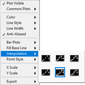
Typically, binned decays are provided as pairs of (t, I) values, where t is the bin’s lower bound and I is the total counts in the time interval [t, t+dt], where dt is the bin (or gate) duration. In that instance, the Interpolation style highlighted in the figure above needs to be chosen. If instead the decays are defined with abscissa t corresponding to the bin (or gate) center, the third Interpolation style in the list shown above needs to be selected (or alternatively the 4th one, which does not represent the bin’s width or duration). In the first case, AlliGator internally converts all abscissa t to t + dt/2 before performing the fit. In the second case, no such conversion is performed. In the uncommon case where the abscissa t represents the bin’s upper bound, the 2nd Interpolation style should be selected, which would result in AlliGator internally converting all abscissa t to t - dt/2 before performing the fit.

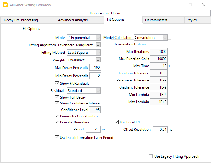
Several fit options, discussed below, are available in the Fit Options panel:

.

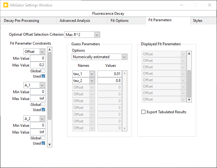
Parameter constraints, guess parameters and whether or not to display the output as plots are managed in the Fit Parameters panel

.

• Fit with constraints applied on individual parameters is handled by an array of Fit Parameter Constraints specifying the:

  • Parameter

  • Min & Max Value

  • whether or not it is a Global parameter (currently unused)

  • whether or not the constraint is Used

• Guess Parameters can be provided in the corresponding array by selecting the parameter name and providing the guess value. Additionally, the way these parameter guesses are used (or not) can be defined via the Options pull-down list:

  • Numerically Estimated

  • User-provided

  • User-provided (normalized)

  • Last valid fitted parameters

• The Displayed Fit Parameters array only applies to series analysis and will be discussed in that context in a later section.

Fit Options Details

• Model: Two models are currently available.

  • A single exponential (1-Exponential) model defined by:

    \(f\left( t \right) = {A_1}\exp \left( { - \frac{t}{{{\tau _1}}}} \right) + b\)

    where b is the baseline and the IRF is offset by an amount (i.e. centered at) \(t_0\).

  • A double exponential (2-Exponentials) model defined by:

    \(f\left( t \right) = {A_1}\exp \left( { - \frac{t}{{{\tau _1}}}} \right) + {A_2}\exp \left( { - \frac{t}{{{\tau _2}}}} \right) + b\)

• Fitting Algorithm: currently, the Levenberg-Marquardt algorithm in the only one implemented.

• Fitting Method: 4 methods are available:

  • Least Square

  • Least Absolute Residuals

  • Bisquare

  • MLE

and the option to try them all out and retain the best:

• Best of All

• Weights: Two types of fits can be performed:

  • Unweighted fit where all data points are equally weighted in the minimization function (sum of difference squared)

  • 1/Variance, where each data point i is weighted by \(1/{f_i}\) (or 1 if \(f_i = 0\)), where \(f_i\) is the function value.

Note

The choice of weights is sometimes a difficult one. Unweighted fits treat departure from the model equally at all points, and thus the residuals with respect to large values (around the decay peak) are those that tend to be minimized best, while the model fit to the tail might not necessarily be good. Inversely, a weighted fit (where the weight is larger the smaller the value is), will tend to minimize the residuals of the function’s tail, allowing for relatively large residuals at the peak. If both fits are visually bad (which is not always adequately reflected in the \(\chi^2\)), something is wrong with the model, the IRF, or the assumption that decay variance is approximately Poissonian is invalid. Or the convergence may have failed, in which case providing reasonable guess parameters might improve the outcome.

• Residuals: The fit residuals (difference between the original decay and its fit) can be optionally plotted in addition to the fit itself. Several options can be chosen:

  The Standard residual is the mere difference between the original decay and its fit, while the Normalized residual is the difference divided by the function value. The Reduced residual is the difference divided by the square root of the absolute value of the function value.

• Min & Max Decay Percentile: The fit can be performed over the whole decay or limited to the “tail” part of the decay. The latter is defined as the part of the decay located between XX% of the decay maximum (max percentile) and YY% (\(0 \le YY < XX \le 100\)) of the decay maximum (min percentile).

• Show Full Decay: When only part of the decay is fitted, it is possible to show the fitted curve (and residuals, optionally) calculated over the full decay range by checking this checkbox. The default (unchecked) is to only show the decay over the selected range.

• Show Confidence Interval: When selecting this option, the confidence interval for each fitted decay value is plotted as two curves (upper limit and lower limit) connected by a colored area.

• Confidence Level: value between 0 and 100.

• Parameter Uncertainties: are estimated from the covariance matrix of all parameters.

• Periodic Boundaries: This option enforces periodic boundary conditions, which is the default situation. The laser repetition period can be entered in the Period box below or the Use Data Information Laser Period checkbox can be checked off.

• Model Calculation: Currently only a Convolution approach is available. It is based on FFT and works best with an IRF covering the whole laser period.

• Termination Criteria: These parameters provide some control over the way convergence of the Levenberg-Marquardt (LM) algorithm is assessed.

  • Max Iterations: This controls the number of iterations of the LM algorithm to perform before stopping optimizing the cost function for a given offset parameter.

  • Max Function Calls: controls the number of calls to the code computing the model values and/or its derivatives. This number is generally close to twice the previous one.

  • Max Time: sets the maximum time spent iterating the LM algorithm.

  • Function Tolerance: Minimum relative change in cost function to achieve in order to stop the LM algorithm.

  • Parameter Tolerance: Minimum relative change in any of the model parameters to stop the LM algorithm.

  • Gradient Tolerance: Minimum relative change in the RMS of the model function’s gradient.

  • Min & Max Lambda: Min & Max value of the LM algorithm’s scale parameter.

• Use Local IRF: When a set of local (or individual) IRFs has been defined, instructs the software to use it (rather than a common IRF defined by the user in the Decay Graph).

• Offset Resolution: The (IRF time) offset parameter is treated separately from the other model parameters. All values in the specified constraint range are tried by stepping through in increment of Offset Resolution, in order to obtain the value for which the fit of the other parameters results in the minimal \(\chi^2\) (or maximal \(R^2\), depending on the Optimal Offset Selection Criterion option discussed next). A small value of this parameter may increase the precision of that parameter but will result in a longer fit duration (which also depends on the Min and Max offset values specified in the constraints array (see below).

Fit Parameters

• Optimal Offset Selection Criterion: When the Offset parameter is fitted (which requires selecting it in the Fit Parameter Constraints array discussed below), the optimal offset is defined as either that for which the \(\chi_2\) is minimized or the \(R^2\) is maximized (which is usually equivalent).

• Fit Parameter Constraints: Fit parameters can be constrained within a specified range defined by the min (-Inf if unconstrained) and max value (Inf if unconstrained).

The list of actual parameters that can be constrained depends on the chosen model:

For instance, choosing \(tau_2\) as a constrained parameter in a 1-Exponential model will have no effect.

If a parameter is unconstrained, it is possible to remove it from the array of constrained parameters by right-clicking on it and choosing Delete Element. If no parameter is constrained, it is possible to delete all elements of the array by right-clicking on the scrollbar and choosing Empty Array. Alternatively, checking off the Used checkbox will ignore this constraint.

Note

If the Offset parameter is fitted, an additional control will be displayed at the top: Optimal Offset Selection Criterion allows defining whether the maximum \(R^2\) or the minimum \(\chi^2\) are used to find the optimal offset parameter. The offset parameter is treated separately from the other parameters: a fit of all the other parameters is performed for a series of Offset values covering the selected constraint range and separated by Offset Resolution.

• Guess Parameters: Convergence of the LM algorithm can sometimes be sped up by providing guesses for one or more parameters of the model. Note that bad guesses can also throw the algorithm off track and prevent obtaining a good fit. Regardless, the algorithm requires starting values for all parameters. There are a few options to provide those:

  • Numerically estimated: simple guesses based on the decay curve are computed for all parameters

  • User-provided: user-provided values are used for parameters that have them, numerically estimated ones for the others.

  • User-provided (normalized): parameters are provided for the normalized decay (for which the maximum value is 1). This allows providing relative amplitude values rather than absolute ones. This is useful when performing multi-ROI NLSF analysis, where the amplitude may vary from ROI to ROI, but the relative amplitude is expected to be fairly constant.

  • Last valid fitted parameters: uses the last successful fit parameters.

• Displayed Fit Parameters: When performing a Series fit, this array determines which fit parameters are output as a plot in the Lifetime & Other Parameters graph. Leave the array empty for all parameters to be output.

Fit Results

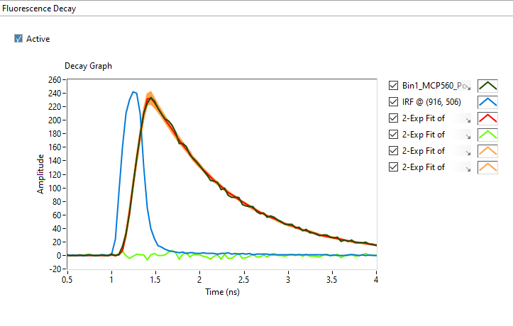
In addition to the plot output(s) in case of a successful fit (see example above), the fit results are output to the Notebook. A typical output will read:

2-Exponential weighted fit of XXXXX

Model Calculation: Convolution
Use Local IRF: TRUE

Periodic with (SYNC) period: 12.5 ns
CPU: 0.655846 s
Fit range: 0%-100%
Fitting Algorithm: Levenberg-Marquardt
Fitting Methods: Least Square
Number of offset fits: 0
Statistics on all offset fits:
Total number of iterations: 1122
Max number of iterations: 1122 [<1000 per fit]
Total number of function calls: 1128
Max number of function calls: 1128 [<10000 per fit]

Gradient: 0 [1E-9]
|Delta Chi2|: 5.748458E-5
|Delta Chi2|/Chi2: 7.149123E-7 [1E-9]
Max |Delta a/a|: 0.00141 [1E-9]
Lambda: 0.001188 [1E-9, 1E+9]
Termination criterion: Max Iterations Exceeded
Residual Sum of Squares (RSS): 710.648673
Akaike Information Criterion (AIC): 2282.215104
Bayesian Information Criterion (BIC): 2359.249576
IRF Normalization Factor: 376.705174
Decay Normalization Factor: 270.8
Guess Fit Parameters:
Type: Numerically estimated
Offset: 0
Baseline: 0
A1: 117
tau 1: 0.981033
A2: 117
tau 2: 2.943098

Fitted Parameters:
Offset: 0.04 ± 0 [0, 0.2] (step: 0.04)
Baseline: -0.387295 ± 0.005974 ]-Inf, +Inf[
A1: 3178.652965 ± 5.446762 [0, Inf]
tau 1: 0.015512 ± 0.010178 ]-Inf, +Inf[
A2: 319.412135 ± 12963.870285 [0, Inf]
tau 2: 0.84741 ± 0.023186 ]-Inf, +Inf[
Amplitude-averaged lifetime: 0.091474
Intensity-averaged lifetime: 0.719217
R^2: 0.998958
Weighted Chi^2: 80.407879
Degrees of freedom: 196
Reduced Weighted Chi^2: 0.410244
Unweighted Chi^2: 710.648673
Reduced Unweighted Chi^2: 3.625759
Standard residuals
Plot(s) added to Decay Graph: 2-Exp Fit of XXXXX, 2-Exp Fit of XXXXX
Residuals, 2-Exp Fit of XXXXX CI Upper Limit, 2-Exp Fit of XXXXX CI Lower
Limit

The first line indicates the fit model (1-Exponential or 2-Exponential) and whether the cost function was weighted or unweighted. XXXXX is the decay name.

Model Calculation indicates how the fitted function is evaluated (currently, the only supported method is by Convolution of the model function with the IRF (when provided). This convolution is done with a normalized IRF (normalized to an integral of 1) such that prescaling (e.g. normalizing) the IRF has no effect on the results. Cyclic convolution is done using Fast Fourier transforms.

Use Local IRF indicates the option selected in the Settings window.

If the Offset parameter is fitted, Number of offset fits indicates how many values have been tested. The following lines indicated the cumulated number of iterations and functions calls used during these different minimizations.

The next section returns minimization parameters for the optimal offset found and what caused the end of iterative minimization. Statistical criteria useful to compare models are provided next (RSS, AIC and BIC).

The IRF Normalization Factor is the integral of the IRF used internally.

Decay Normalization Factor is the corresponding integral of the decay, used to normalize the decay internally before computation.

\(R^2\) as well as the 68% confidence intervals (errors) are defined according to this page. The weighted \(\chi ^2\) is defined as the Sum of Squares Error (SSE) defined on that page, with weights equal to \(1/y_i\), where \(1/y_i\) is the local function value, while the unweighted \(\chi ^2\) is defined similarly but with uniform weights equal to 1. The appropriate \(\chi ^2\) to consider depends on the type of fit (for instance, the weighted \(\chi ^2\) is the one relevant in this example). The alternative \(\chi ^2\) is provided for comparison. Reduced \(\chi ^2\) are obtained by dividing the previous quantities by the number of Degrees of freedom. A reasonable fit with Poisson uncertainties on the decay values will have a reduced weighted \(\chi ^2\) close to 1.

If the fit fails, an error message will be displayed instead (and not plot will be added to the Decay Graph).

Multiple ROIs decay fit

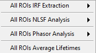
It is possible to fit multiple ROI decays in a single action, using one of the options of the Analysis:FLI Dataset:Multiple ROIs Analysis menu. The analysis applies to all ROIs currently defined in the Source Image.

.

There are two possible options:

• Use a common IRF for all ROIs: the IRF needs to be defined using the IRF/Reference Plot:Use as IRF/Reference Plot menu item of the Decay Graph.

• Use one IRF per ROI: this option is recommended when the IRF is known to depend on the location in the field of view, as is for instance often the case with wide-field detectors.

Additionally, there are two types of outputs depending on the chosen mode (verbose or silent, or equivalently slow or fast), which are described next.

• Slow mode: In this case, each ROI decay is output to the Decay Graph, as well as the corresponding fit and residuals curves. The fit results are sent to the Notebook, as would happen in an interactive approach. While this provides visual feedback to the user, it is memory and time consuming, and is not the recommended approach in general.

• Fast mode: In that case, no decay, fit or residuals curve is output in the Decay Graph, and instead the results are stored internally and optionally exported as an ASCII file if the Export Tabulated Results checkbox in the Settings:Fluorescence Decay:Fit Parameters panel is checked off. The fit results can be examined using the Decay Fit Parameter Map panel, as discussed in the corresponding manual page.

In order to define individual IRFs, use the Analysis:FLI Dataset:Multiple ROIS Analysis:All ROIs IRF Extraction menu. An IRF dataset file is needed for that purpose, which is usually obtained with a solution of quenched fluorescent dye, laser reflection off of a piece of paper or mirror, or any other method resulting in data reporting on the temporal profile of the setup’s response.

There are again two options (slow and fast) to extract these IRFs, the first one outputting the different IRFs to the Decay Graph, while the latter stores data internally. One of AlliGator’s status LEDs at the bottom right of the window turns on when local IRFs have been defined.

In order to take advantage of these stored IRFs, it is necessary to check off the Use Local IRF checkbox in the Settings:Fluorescence Decay:Fit Options panel.

The Local IRFs computed in this manner can be saved to (HDF5) file using the Analysis:FLI Dataset:Multiple ROIS Analysis:All ROIs IRF Extraction:Save Local IRFs menu item. They can later be reloaded using the corresponding Analysis:FLI Dataset:Multiple ROIS Analysis:All ROIs IRF Extraction:Load Local IRFs menu item.

To clear these IRFs from memory, use the Analysis:FLI Dataset:Multiple ROIS Analysis:All ROIs IRF Extraction:Clear Local IRFs menu item.

Series decay fit

In the case of a series analysis, decay fits can be performed by choosing FLI Dataset Series:Series NLSF Analysis:Current ROI or Sequential ROIs in the Analysis:FLI Dataset Series menu. The two options work as follows:

• Current ROI: the current

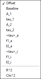
Each time point decay is fitted separately, following the protocol described previously for single decays. In addition, it is possible to generate one or more plots of the evolution of selected fit parameters across the series, using the Displayed Fit Parameters array. These plots will be output in the Lifetime & Other Parameters Graph of the Lifetime Analysis panel (see the corresponding manual page ). Parameters that can be displayed can be chosen from the following list:

.

This list includes the fit parameters and derived quantities, such as the mean lifetimes <tau>_a and <tau>_i or fractions f1_a and f1_i (for the 2-Exponentials model, defined below), or the \(R^2\) and \(\chi ^2\) outputs.

amplitude-averaged lifetime	intensity-averaged lifetime
\(\left\langle \tau \right\rangle_a = f_{1a}\tau _1 + f_{2a}\tau _2\)	\(\left\langle \tau \right\rangle_i = f_{1i}\tau _1 + f_{2i}\tau _2\)
\(f_{1a} = \frac{A_1}{A_1 + A_2}\)	\(f_{1i} = \frac{{{A_1}{\tau _1}}}{{{A_1}{\tau_1} + {A_2}{\tau_2}}}\)
\(f_{2a} = 1 - f_{1a}\)	\(f_{2i} = 1 - f_{1i}\)

Note that the above definitions are only valid in the approximation of large laser period (compared to the respective lifetimes). The exact formulas are:

amplitude-averaged lifetime	intensity-averaged lifetime
\(\left\langle \tau \right\rangle_a = f_{1a}\tau _1 + f_{2a}\tau _2\)	\(\left\langle \tau \right\rangle_i = f_{1i}\tau _1 + f_{2i}\tau _2\)
\(f_{1a} = \frac{A'_1}{A'_1 + A'_2}\)	\(f_{1i} = \frac{{{A'_1}{\tau _1}}}{{{A'_1}{\tau_1} + {A'_2}{\tau_2}}}\)
\(A'_i = A_i \left(1 - \exp{(-T/\tau_i)} \right)\), i = 1 or 2	\(A'_i = A_i \left(1 - \exp{(-T/\tau_i)} \right)\), i = 1 or 2
\(f_{2a} = 1 - f_{1a}\)	\(f_{2i} = 1 - f_{1i}\)

(last modified on 01-30-2026)