Settings Window¶

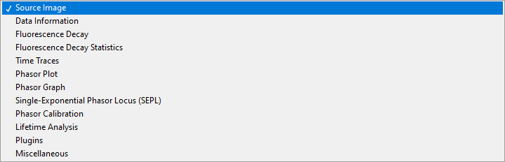
The Settings window can be opened via the Windows:Show Settings menu item (Ctrl+E shortcut) in the main AlliGator window. It is comprised of multiple pages and sub-pages, which can be accessed via the top page selector:

The different pages are described in the sections below. Note that any value change done in the Settings window immediately takes effect and is reflected in the corresponding AlliGator window control (if there is one).

Inversely, any change to a control in the AlliGator window is immediately reflected in the Settings window.

The value of the Settings controls are saved when AlliGator quits, and reloaded when it is restarted.

Source Image¶

The Source Image panel is comprised of 3 sub-panels:

Use Image Histogram for Contrast: if checked, uses the location of the Min and Max cursors in the Image Histogram to adjust the correspondence between pixel intensity and color scale. Namely, any pixel with intensity smaller than Min will be colored with the Low Color shown below the color scale, while any pixel with intensity larger than Max will be colored with the High Color shown above the color scale. Pixels with intensity between Min* and Max will be colored according to the color scale.

A side effect of this selection is that, when hovering over the image, the indicated intensity will show clipped values, any pixel with intensity smaller than Min will be indicated as equal to Min, while any pixel with intensity larger than Max will be indicated as equal to Max. However, internally, the correct intensity value is preserved. To read the actual intensity of a pixel, simply unchecked this option before hovering over the pixel again.
Low Count Pixels Rejection Options: defines which rejection criteria to use for the dimmest pixels in the image. The minimum of all criteria, \(m = Min(Min_B, Min_T, Min_P)\), is used.
- Reject Low Count Pixels: when checked off, combine the following criteria to define a minimum value \(m\).the pixel intensity \(I\) needs to reach in order to be included in subsequent analyses: \(I \ge m\).
- Background Low Threshold Factor: this factor (\(b\)) is multiplied by the mode \(M\) of the image histogram (computed with 256 bins) to obtain \(Min_B = b M\).
- Fixed Low Background Threshold: fixed quantity \(Min_T\), for instance estimated using the Min cursor of the Image Histogram to highlight pixels in the image below that value.
- Low Percentile: value \(P_{min}\) defining \(Min_P\) such that \(P_{min}\) percent of all pixels have intensity \(I \ge Min_P\).
High Count Pixels Rejection Options: defines which rejection criteria to use for the brightest pixels in the image. The maximum of all criteria, \(M = Max(Max_B, Max_T, Max_P)\), is used.
- Reject High Count Pixels: when checked off, combine the following criteria to define a maximum value \(M\).the pixel intensity \(I\) needs to reach in order to be included in subsequent analyses: \(I \le M\).
- Background High Threshold Factor: this factor (\(B\)) is multiplied by the mode \(M\) of the image histogram (computed with 256 bins) to obtain \(Max_B = B M\).
- Fixed High Background Threshold: fixed quantity \(Max_T\), for instance estimated using the Max cursor of the Image Histogram to highlight pixels in the image above that value.
- High Percentile: value \(P_{max}\) defining \(MaxP\) such that \(P_{max}\) percent of all pixels have intensity \(I \le Max_P\).
Hot Pixel Removal: options used to replace “screamers” in SPAD arrays by the median value of neighboring pixels (requires reloading the dataset to take effect).
- Remove Hot Pixels: when checked off, applied hot pixel removal algorithm.
- Percentile: percentile of high intensity pixels to consider as hot pixels.
- Use Hot Pixel Mask: when checked off, ignores the Percentile parameter and used the Hot Pixel Mask Image instead.
- Hot Pixel Mask Image: path of the mask (binary) image identifying hot pixels.

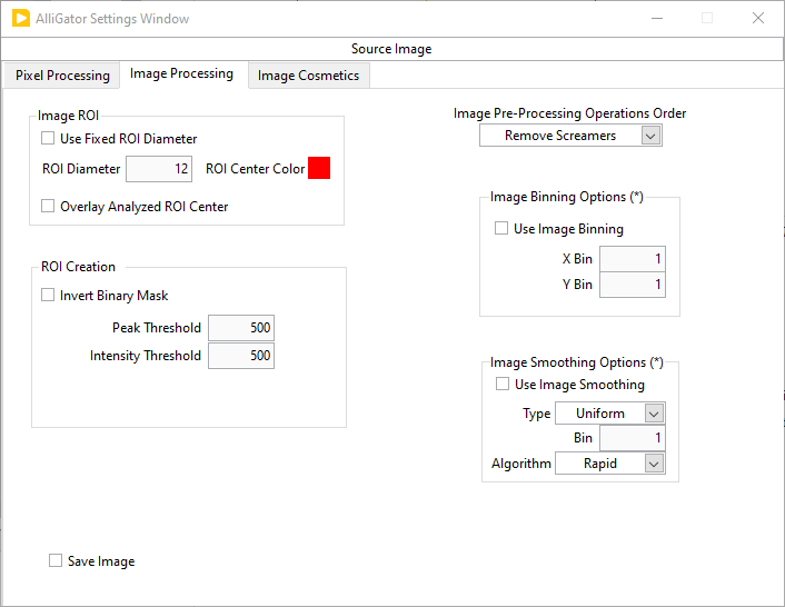
_images/AlliGator-Settings-Source-Image-Processing.png

Image ROI options
- Use Fixed ROI Diameter: when checked off, forces circular ROIs to adopt the specified diameter (see next).
- ROI Diameter (in pixel): used in conjunction with the previous option.
- ROI Center Color: used to locate the center of the last ROI whose decay was processed (interactive mode only).
- Overlay Analyzed ROI Center: if checked off, the center of the analyzed ROI is highlighted using the
ROI Creation
- Invert Binary Mask: check off this box to use binary mask images with regions of interest labeled with a value larger than the background.
- Peak Threshold: Min parameter used in the “Create ROI(s) from Pixels with Peak above Min” right-click menu function of the Source Image.
- Intensity Threshold: Min parameter used in the “Create ROI(s) from Pixels with Intensity above Min” right-click menu function of the Source Image.
Image Pre-Processing Operations Order: ordered drop-down list of operations (optionally) applied to each gate image. Right-click on the list to access the Reorder Operations dialog window.
Image Binning Options: requires reloading the current dataset to be applied.
- Use Image Binning: check off this box to apply binning to gate images.
- X/Y Bin*: binning parameter for each dimension.
Image Smoothing Options: requires reloading the current dataset to be applied.
- Use Image Smoothing: check off this box to apply smoothing to gate images.
- Type:
  - Uniform: each pixel is replaced by an average of itself and its neighbors.
  - Bilinear: each pixel is replaced by a weighted average of itself and its neighbors, the weights decreasing linearly from 1 away from the center (to zero for the pixels outside the kernel dimension).
  - Gaussian: each pixel is replaced by a weighted average of itself and its neighbors, the weights decreasing according to a Gaussian width \(\sigma = Bin/6\) from 1 away from the center.
- Bin: kernel dimension used in the smoothing operation.
- Algorithm:
  - Rapid: ignores image border subtleties.
  - Thorough: treats borders properly but can be significantly slower for large datasets.
Save Image: check off this box to save the displayed image with its overlay each time a new dataset is loaded. The file is saved in the Saved Displayed Image Format specified in the Miscellaneous Settings panel, in the same folder as the current dataset, with the dataset name to which the image type (Gate n, White Light or Total Intensity) is appended.

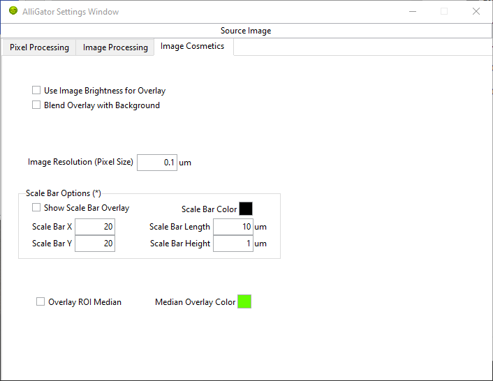
_images/AlliGator-Settings-Source-Image-Cosmetics.png

Use Image Brightness for Overlay: when used, this option scales the pixel overlay color by the factor \(\lambda = (I - range_{min})/(range_{max} - range_{min})\), where I is the pixel’s intensity.
Blend Overlay with Background: when used, this option replaces the pixel overlay color by \(\lambda O + (1-\lambda) B\), where O is the unscaled overlay color and B the underlying pixel color according to the source image color scale.
Image Resolution (Pixel Size): information used to overlay a scale bar on the image (see Scale Bar Options below).
Scale Bar Options: requires reloading the image or clicking the Scale Bar Overlay button on the Source Image panel.
- Show Scale Bar Overlay: check this off to automatically show the scale bar when loading a new dataset.
- Scale Bar X/Y: location of the scale bar in pixel unit. X = 0 corresponds to the left of the image. Y = 0 corresponds to the top of the image.
- Scale Bar Length/Height: dimension of the displayed scale bar in physical units.

Data Information¶

The options in this panel are discussed in the Data Information section of the Loading & Saving FLI Datasets page.

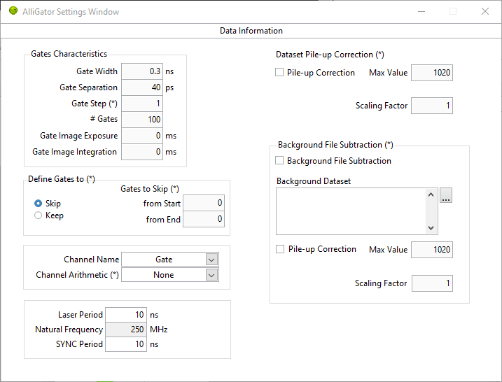
Gate Characteristics: loaded with the dataset file, although in some cases (e.g. raw .ptu files), the # Gates can be specified before loading. These parameters can be overwritten after loading, for instance to correct for a known bogus parameter value.
- Gate Width: for a square gate (or bin), defines the nominal full width at half maximum (FWHM). For binned data, it is the bin size.
- Gate Separation (or gate shift): temporal offset of two consecutive gates. In the case of binned data, this parameter is equal to the Gate Width parameter.
- Gate Step: integer parameter specifying by how much the index of successive gates is incremented when loading a new dataset. The default is 1, which corresponds to all gates being loaded. A value of 2 would result in every other gate being loaded.
- # Gates: number of gates in the dataset (or number of gates to bin the data into in the case of a time-tagged dataset such as .ptu files). For dual-gate datasets, this corresponds to the number of channel pairs.
- Gate Image Exposure: time during which the detector is actually capable of detecting photons (= n x W, where n is the number of laser periods and W the gate width).
- Gate Image Integration: total time taken to acquire the gate image (= n x T, where n is the number of laser periods during acquisition and T is the laser period).
Define Gates to: Skip or Keep, whose corresponding parameter are displayed below, allows to reject gates when loading a dataset, providing two alternative ways to do so:
- Gates to Skip: from Start/End are the number of gates to ignore at the beginning/end of the series when loading the dataset.
- Gates to Keep*: First/Last are the indices of the first (default: 0) and last gate (default: 4294,967,295) to keep when loading the dataset. The indice of the first gate in the dataset is 0, while the index of the last gate is G-1, where G is the total number of gates in the dataset.
Channel Name: List showing the root name of available gates in the loaded dataset. For standard single channel datasets, this will be limited to a single name (generally Gate), while in the case of dual-channel datasets, the name of both channels will be shown. Use this drop-down list to switch from one to the other and update the displayed Source Image.
Channel Arithmetic: “None”/”INT-G2”/”G2/INT*<INT>”/”(1-G2/INT)*<INT>” is a list allowing to process and display arithmetic combinations of dual-channel gates. It is necessary to reload the dataset to apply this change. Note that, unless None is selected, changing the Channel Name parameter will have no effect on the displayed Source Image.
Laser Period: generally loaded from the dataset when available. Can be user-modified
Natural Frequency: indicator representing 1/D, where D is the duration covered by the loaded gates. It is the recommended frequency for phasor analysis.
SYNC Period: in general it is identical to the laser period (or undefined). It is the trigger frequency used during gate acquisition. When SYNC Period > Laser Period, multiple decay periods can be expected in the data.
Dataset Pile-up Correction options: the type of corrected pile-up is that experienced in photon-counting detectors with finite counting capabilities. The correction is applied on each loaded dataset as part of a series of operations whose order is defined in the Source Image:Image Processing panel Image Pre-Processing Operations Order list.
- Pile-up Correction: check off this box to apply pile-up correction.
- Max Value: maximum value obtainable in each pixel.
Scaling Factor: optional dataset gate image intensity scaling factor (default: 1).
Background File Subtraction options:
- Background File Subtraction: check off this box to apply background file subtraction when loading a dataset.
- Background Dataset: path of the dataset used as background file.
- Pile-up Correction: whether or not to apply pile-up correction as part of the background dataset loading steps.
- Max Value: maximum value obtainable in each pixel.
- Scaling Factor: optional dataset gate image intensity scaling factor (default: 1).

Fluorescence Decay¶

The Fluorescence Decay tab is divided into 5 sub-panels:

Decay Pre-Processing
Advanced Analysis
Fit Options
Fit Parameters
Styles

described below.

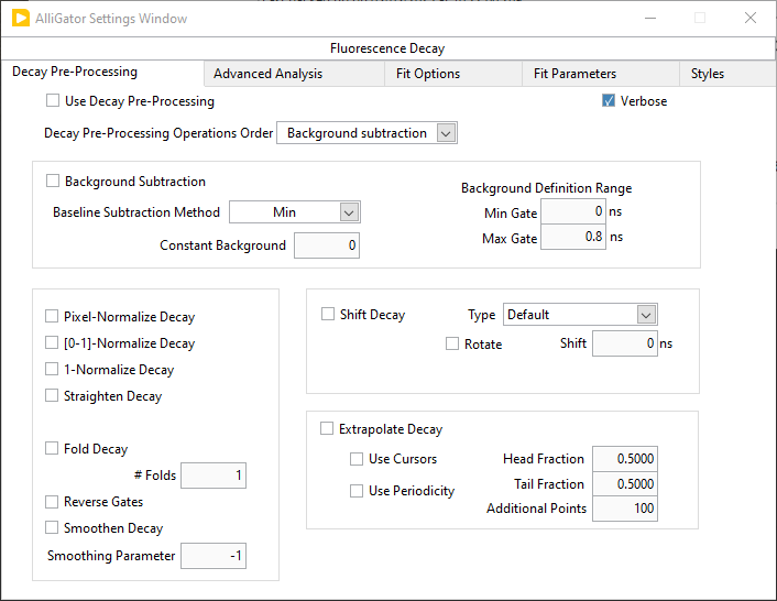
Decay Pre-Processing¶

The options exposed in this panel are discussed in the Decay (Pre-) Processing page of the manual.

Advanced Analysis¶

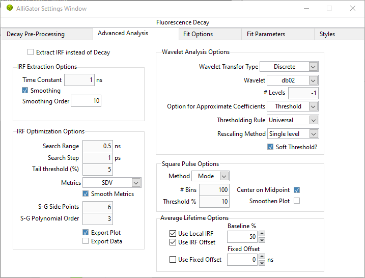
Extract IRF instead of Decay: in interactive mode, follows the Analysis:FLI Dataset:Current ROI Analysis step with a deconvolution step using the IRF Extraction Options, and outputs the resulting computed IRF instead of the decay.

IRF Extraction Options¶

Time Constant: single-exponential time constant used for deconvolution.
Smoothing: applies one or more iterations of a Savitzky-Golay filter (6 side points, polynomial order 3) to the deconvolved IRF.
Smoothing Order: number of iterations of the Savitzky-Golay filter.

IRF Optimization Options¶

Parameters for the optimal IRF extraction algorithm. The center lifetime \(\tau_0\) used in the search is the Time Constant parameter of the IRF Extraction Options.

Search Range: \(\Delta \tau\) defines the half search interval in which the optimal time constant is searched for.
Search Step: \(\delta \tau\) is the step size by which the trial time constant is incremented at each step of the search.
Tail Threshold (%): percentage of the deconvolved IRF tail used to compute the metrics.
Metrics: quantity used to determine the optimal time constant for deconvolution.
Smooth Metrics: if checked, a Savitzky-Golay filtered metrics is used to find the optimum time constant for IRF deconvolution
S-G Side Points: number of side points used to compute the Savitzky-Golay filtered metrics.
S-G Polynomial Order: polynomial order used to compute the Savitzky-Golay filtered metrics.
Export Plot: if checked, sends the metrics plots (raw and filtered) to the Notebook.
Export Data: if checked, sends the metrics values to the Notebook

Wavelet Analysis Options¶

The Wavelet Analysis Options are used to denoise decays (Decay Graph’s Process Plot(s):Denoising right-click menu). The parameters and their interpretation are described in the online LabVIEW Advanced Signal Processing Toolkit manual (https://www.ni.com/docs/en-US/bundle/lvaspt-api-ref/page/vi-lib/addons/wavelet-analysis/application-llb/wa-denoise-vi.html)

Specifically, the Wavelet Transform Type parameter allows selecting between a Discrete Wavelet Transform (https://www.ni.com/docs/en-US/bundle/lvaspt-api-ref/page/vi-lib/addons/wavelet-analysis/application-llb/wa-denoise-dwt-real-array-vi.html) and a “Undecimated Wavelet Transform* (https://www.ni.com/docs/en-US/bundle/lvaspt-api-ref/page/vi-lib/addons/wavelet-analysis/application-llb/wa-denoise-uwt-real-array-vi.html).

Square Pulse Options¶

These options are used for fits of the decay to a square pulse or its variants (logistic square pulse and tilted logistic square pulse).

Method: Mean or Median, refers to the algorithm used to determine the baseline (low level) and plateau (high level) values used to define the square wave.
# Bins: number of bins used to compute the level histogram used to determine the low and high level of the square pulse.
Threshold %: percentage of the low-to-high level height used to define the rising and falling edges start and stop.
Center on Midpoint: defines whether the rising and falling edges of the “square” pulse pass through the rising and falling edges midpoints.
Smoothen Plot*: defines whether the decay is smoothened before being fitted to a square pulse.

Average Lifetime Options¶

These options define the way an estimate of the average lifetime is computed based on the measured decay and the IRF.

Use Local IRF: used only for multi-ROI analysis.
Use IRF Offset: define the decay offset as that deduced from the IRF according to the:
Baseline %: define a threshold th = (1 + %) x baseline and find its intersection with the rising edge of the IRF as illustrated below.

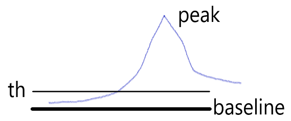
Use Fixed Offset: ignoring the IRF, define a fixed offset to define time 0 of the decay.

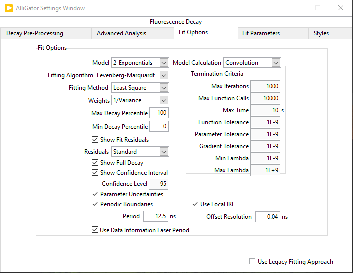
Fit Options¶

The options accessible on this panel are discussed in the Single decay fit section of the Fluorescence Decay Fitting page of the manual.

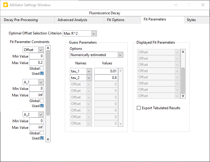
Fit Parameters¶

The parameters accessible on this panel are discussed in the Fit Parameters section of the Fluorescence Decay Fitting page of the manual.

Styles¶

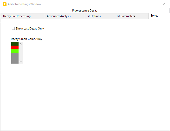
Show Last Decay Only: if checked off, hides all other plots in the Decay Graph when adding a new plot.
Decay Graph Color Array: colors used for the decay itself, its fit and its residuals.

Fluorescence Decay Statistics¶

The Fluorescence Decay Statistics panel of AlliGator provides information on the max and min intensities in each pixel, displaying an histogram of both. The parameters in the corresponding panel of the Settings window allow using this information to reject pixels based on their min and max intensity, similarly to what the Low/High Count Pixels Rejection Options of the Source Image panel allow doing based on the total pixel intensities.

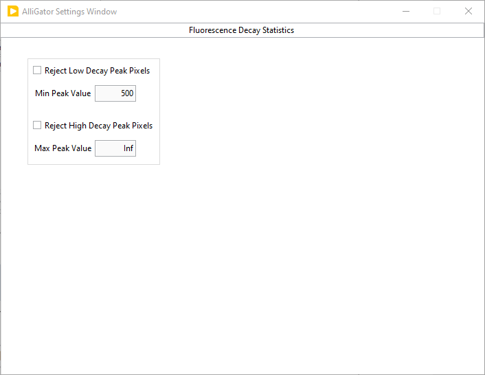
_images/AlliGator-Settings-Decay-Statistics.png

Reject Low Decay Peak Pixels: if checked off, rejects decays whose peak values are strictly smaller than Min Peak Value.
Min Peak Value: peak value lower rejection threshold.
Reject High Decay Peak Pixels: if checked off, rejects decays whose peak values are strictly larger than Max Peak Value.
Max Peak Value: peak value upper rejection threshold.

These criteria are applied after the min and max total intensity constraints defined in the Settings:Pixel Processing panel.

Intensity Time Trace¶

Parameters in this panel affect the way intensity time traces, discussed in the Intensity Time Trace Panel are computed.

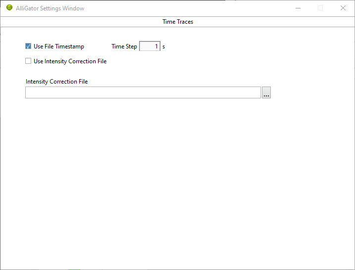
_images/AlliGator-Settings-Time-Traces.png

Use File Timestamp: check off this box to use the timestamp saved with each dataset in a series, when building the intensity time trace.
Time Step: increment used to compute the timestamp of each dataset in a series, absent a timestamp saved with the dataset.
Use Intensity Correction File: Check off this box to renormalize the intensity time with the information contained in the Intensity Correction File.
Intensity Correction File: path of the intensity correction file to be used renormalize the intensity time trace.

Phasor Plot¶

The Phasor Plot panel is subdivided into 3 subpanels:

Phasor Plot Calculation
Phasor Plot Information Overlay
Phasor Plot Appearance

Phasor Plot Calculation¶

The parameters in this panel are used to control the way the phasor plot is computed and represented in the Phasor Plot panel of AlliGator, discussed in the Phasor Plot Panel page of the manual.

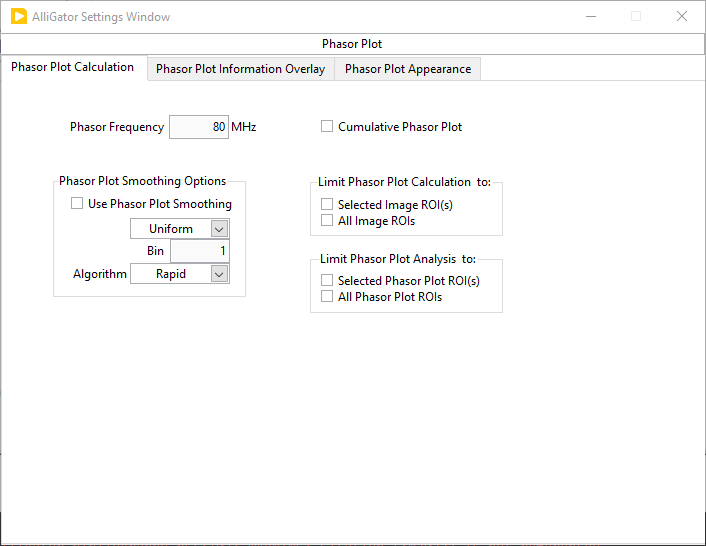
Phasor Frequency: sets the frequency used to compute phasors. This value is synchronized throughout AlliGator different windows and panels.
Cumulative Phasor Plot: check off this box to preserved phasor plot data when loading new datasets. When checked off, the current phasor plot is not preserved. The first phasor plot to be accumulated is the subsequent one.
Phasor Plot Smoothing Options:
- Use Phasor Plot Smoothing: check off this box to apply smoothing to the phasor plot
- Type:
  - Uniform: each phasor is replaced by an average of the phasor of its pixel and those of its neighbors.
  - Bilinear: each phasor is replaced by a weighted average of the phasor of its pixel and those of its neighbors., the weights decreasing linearly from 1 away from the center (to zero for the pixels outside the kernel dimension).
  - Gaussian: each phasor is replaced by a weighted average of the phasor of its pixel and those of its neighbors., the weights decreasing according to a Gaussian width \(\sigma = Bin/6\) from 1 away from the center.
- Bin: kernel dimension used in the smoothing operation.
- Algorithm:
  - Rapid: ignores image border subtleties.
  - Thorough: treats borders properly but can be significantly slower for large datasets.
Limit Phasor Plot Calculation to:
- Selected Image ROI(s): currently limited to a single ROI. All pixels outside the ROI are excluded from the phasor plot calculation.
- All Image ROIs: All pixels outside the image ROIs are excluded from the phasor plot calculation.
Limit Phasor Plot Analysis to:
- Selected Phasor Plot ROI(s): currently limited to a single ROI. When performing an analysis involving the phasor plot data, limits this analysis to the phasors within the selected phasor plot ROI.
- All Phasor Plot ROIs: When performing an analysis involving the phasor plot data, limits this analysis to the phasors within any of the phasor plot ROIs.

Phasor Plot Information Overlay¶

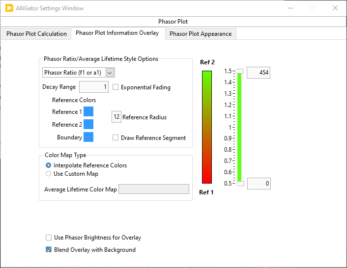
Phasor Ratio/Average Lifetime Style Options:
- Color Map Type:
  Phasor Ratio (f1 or a1): standard phasor ratio (either intensity or amplitude weighted, depending on the Phasor Ratio Type parameter in the Phasor Graph panel of the Settings window).
  
  Average Lifetime (<tau>_i or <tau>_a): amplitude- or intensity-weighted average lifetime, depending on the Phasor Ratio Type parameter in the Phasor Graph panel of the Settings window).
  
  User-Defined Quantity: elementary quantity or alias for a definition based on elementary quantities.
- User-Defined Quantity: Use the context menu of this control to open the Aliases Definitions window and define a quantity based on one of the following elementary quantities:
  f1: phasor ratio
  
  a1: amplitude phasor ratio
  
  tau_phi: phase lifetime
  
  tau_m: modulus lifetime
  
  <tau>_i: intensity-weighted average lifetime
  
  <tau>_a: amplitude-weighted average lifetime
  
  tau_1: lifetime of phasor ratio reference 1
  
  tau_2: lifetime of phasor ratio reference 2
- Decay Range: range of the exponential fading factor used in the phasor ratio (or other derived quantity) color map. This range is shown as a boundary surrounding the two reference phasors in the Phasor Plot. If the Exponential Fading checkbox is not selected, phasors outside the range (i.e. whose distance to the segment connecting the two references is larger than the range) are not taken into account in subsequent analyses.
- Exponential Fading: if checked off, applies an exponentially decaying fading factor to the phasor ratio (or other derived quantity) color map intensity.
- Reference Colors:
  Reference 1: color used for phasor reference 1.
  
  Reference 2: color used for phasor reference 2.
  
  Boundary: color used for the boundary of the region of the phasor plot located Decay Range away from the segment connecting phasor references 1 & 2.
- Reference Radius: size of the dots representing references 1 & 2 on the phasor plot.
- Draw Reference Segment: whether or not to connect both references by a (dashed) line.
- Color Map Type: Interpolate Reference Colors or Use Custom Map.
- Average Lifetime Color Map: right-click on the box to select predefined color scales.
Color Scale: represents the selected Color Map.
Display Range: slide used to define the min and max Phasor Ratio/Average Lifetime/User-Defined Quantity encoded by the Color Scale. The sliders and the corresponding values displayed in the respective numeric controls to the right correspond to the max and min values encoded by the color scale. The max and min values displayed on the left scale have no meaning for the color coding.
Use Phasor Brightness for Overlay: when color-coding the pixels of a ROI in the Source Image, this option allows adjusting the color intensity to the underlying phasor plot bin value.
Blend Overlay with Background: if checked off, this option replaces the black color corresponding to 0-valued bins in the option above by the phasor plot current color.

Phasor Plot Appearance¶

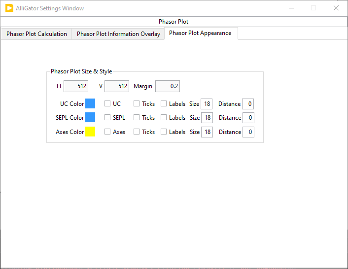
Phasor Plot Size & Style
- H: horizontal size (in pixels) of the phasor plot image.
- V: vertical size (in pixels) of the phasor plot image.
- Margin: fractional size of the regions to the left and right of the unit square in which the universal circle is encompassed.
- UC Style: universal circle style settings.
  UC Color: color used for the UC.
  
  UC: whether or not to display the UC.
  
  Ticks: whether or not to display the phase lifetime ticks.
  
  Labels: whether or not to display the tick labels.
  
  Size: label size in pixels.
  
  Distance: distance of the labels from the UC in pixels.
- SEPL Style: single-exponential phasor locus style settings.
  SEPL Color: color used for the SEPL.
  
  SEPL: whether or not to display the SEPL.
  
  Ticks: whether or not to display the phase lifetime ticks.
  
  Labels: whether or not to display the tick labels.
  
  Size: label size in pixels.
  
  Distance: distance of the labels from the SEPL in pixels.
- Axes Style: axes style settings.
  Axes Color: color used for the axes.
  
  Axes: whether or not to display the axes.
  
  Ticks: whether or not to display the axes ticks.
  
  Labels: whether or not to display the tick labels.
  
  Size: label size in pixels.
  
  Distance: distance of the labels from the axes in pixels.

Phasor Graph¶

The Phasor Graph panel of the Settings window contains options and parameters that have an effect beyond the Phasor Graph panel of AlliGator.

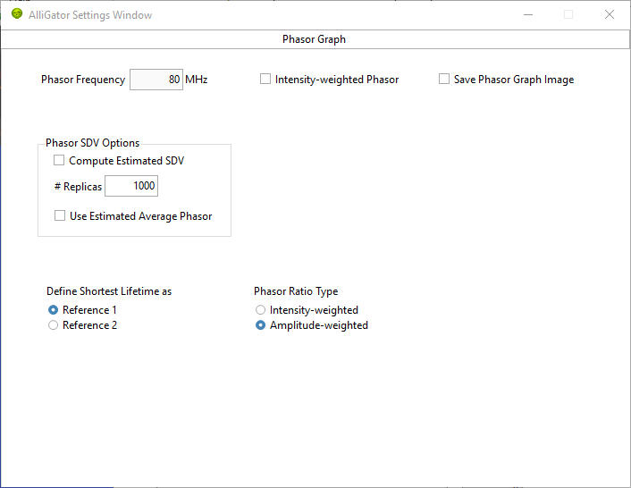
Phasor Frequency: sets the frequency used for phasor computation throughout AlliGator.
Save Phasor Graph Image: if checked off, every change to the Phasor Graph generates a file named “Phasor Graph Current Dataset (n).xxx” in the current dataset folder, where Current Dataset is the file name of the current dataset and n is an integer incremented to avoid overwriting previous files. xxx is the file extension corresponding to the Saved Displayed Image File Format defined in the Miscellaneous Settings panel.
Phasor SDV Options: used in case an estimate of the shot noise contribution to the phasor (and average lifetime) standard deviation needs to be estimated.
- Compute Estimated SDV: turns the option on or off.
- # Replicas: number of replicas of the decay simulated to estimate the phasor SDV.
- Use Estimated Average Phasor: if checked off, returns the average of all replicas instead of the original phasor.
Define Shortest Lifetime as: Reference 1/Reference 2: when computing phasor references, defines the shortest lifetime as the selected reference.
Phasor Ratio Type: Intensity-Weighted/Amplitude-weighted: specifies which phasor ratio (or derived quantity such as the average lifetime) to compute.

Single-Exponential Phasor Locus (SEPL)¶

The options and parameters in this panel control the aspect of the SEPL as displayed in the Phasor Plot image or the Phasor Graph. For a detailed explanation of the role of these different parameters, check ref. [XM21] in the Bibliography page.

Display¶

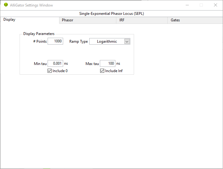
Display Parameters:
- # Points: number of points used to draw the SEPL.
- Ramp Type: Linear/Logarithmic.
- Min tau: lower \(\tau\) value used in the ramp.
- Include 0: whether or not to add the phasor for \(\tau = 0\)
- Max tau:upper \(\tau\) value used in the ramp.
- Include Inf: whether or not to add the phasor for \(\tau = \inf\)

Phasor¶

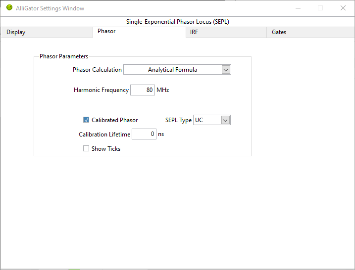
Phasor Parameters:
- Phasor Calculation: Direct Sum/Analytical Formula
- Harmonic Frequency: frequency used to compute the SEPL. This is not linked to the Phasor Frequency parameters visible in the Phasor Plot and Phasor Graph panels of the Settings and AlliGator windows.
- Calibrated Phasor: if checked off, calibrate the SEPL using the remaining parameters.
- SEPL Type: UC/L_N/L_N(W)/L_X
- Calibration Lifetime: self-explanatory.
- # Gates: number of gates used to compute the calibration phasor.
- Show Ticks: shows ticks on the computed SEPL

IRF¶

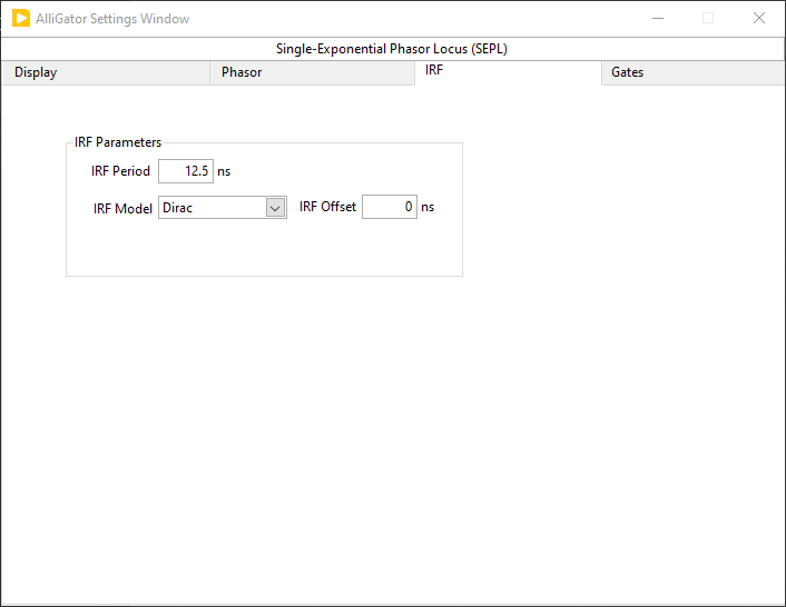
IRF Parameters:
- IRF Period: self-explanatory.
- IRF Model: Dirac/Exponential
- IRF Offset: time shift of the IRF.

Gates¶

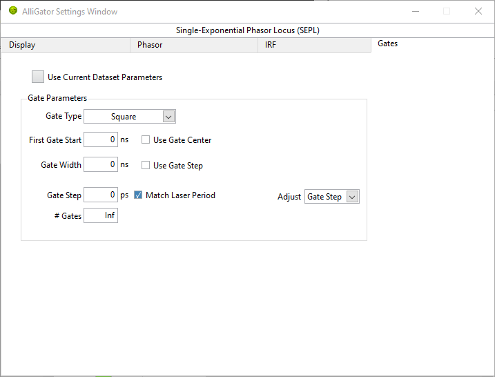
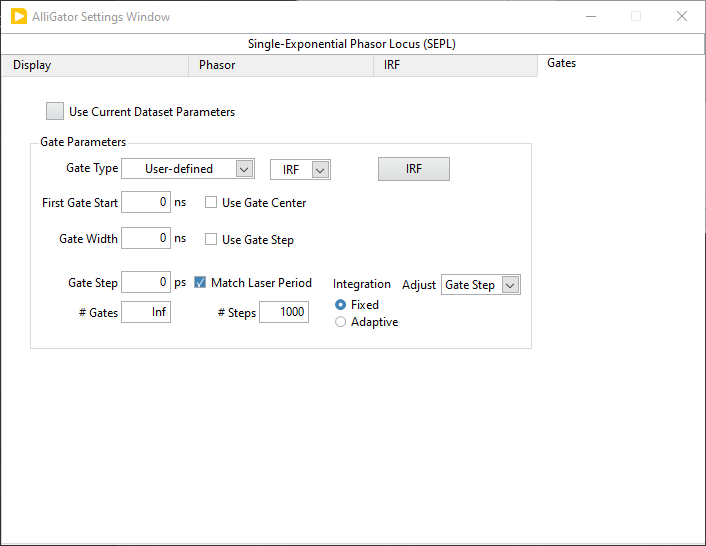
Use Current Dataset Parameters: if checked off, use the gate parameters of the current loaded dataset, as defined in the Data Information panel.
Gate Parameters:
- Gate Type: select what type of gate shape is used.
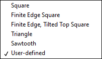
- Type of User-defined Function: Gate/IRF
- Edit User-defined Function: button used to open the Plot Editor window in which to load or define the function to use.
- First Gate Start: location of first timestamp.
- Use Gate Center: if checked off, timestamps indicate the center of the gate rather than its start.
- Gate Width: self-explanatory.
- Use Gate Step: if checked, the width is equal to the gate step.
- Gate Step: separation between consecutive gates
- Match Laser Period: if checked, indicates that the series of gates covers the whole laser period.
- Adjust: Gate Step/# Gates. Shown when Match Laser Period is selected.
- # Gates: number of gates comprising the waveform.
- Integration: Fixed/Adaptive. shown when User-defined Gate Type is selected. Specifies how the resolution used for convolution is defined.
- Tolerance: shown when Adaptive Integration is selected.
- # Steps: shown when Fixed Integration (step number) is selected. Number of integration steps used for convolution.

Phasor Calibration¶

Calibration Options:
- Calibration Lifetime: single-lifetime lifetime of the decay used as calibration phasor.
- Calibration Type: None/Single Phasor/Phasor Series/Phasor Map
- Use Backup Calibration if needed: check this box off to use backup a calibration phasor if none is available. The type of backup calibration phasor used is defined by Backup Calibration Type.
- Backup Calibration Type: if there is no calibration phasor defined for a dataset in a series, and Use Backup Calibration if needed is checked off, the backup calibration used instead can be of two types:
  Single Calibration: uses the Single Calibration phasor stored internally (if one has been defined). If none, has been defined, no calibration is used.
  
  Nearest Valid Calibration: looks for the closest valid calibration available in the series. If none is found, uses the single calibration phasor stored internally, or no calibration if none has been defined.

Lifetime Analysis¶

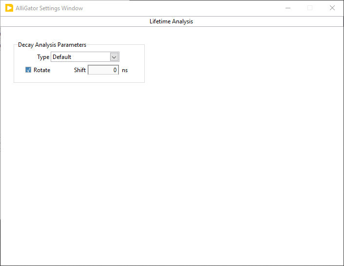
Decay Analysis Parameters
- Type: Default/CDF/Threshold/Cross-Correlation selects which lifetime-related quantity is computed when using the Compute Single Phasor Ratio at Mouse Location menu item in the Phasor Graph. Default corresponds to the average lifetime, while the other three options correspond to the decay offset with respect to the stored IRF/Reference Decay.
- Shift: used in the CFD case (Constant Fraction Discrimination), where a shifted inverted decay is used.

Plugins¶

Python Settings:
- Python Version: Python version called when using a plugin. The example scripts have been tested with Python 3.9, but it is likely that calls to later (and possibly earlier) versions might work.
- Use PATH definition: if checked off, used the PATH system file to obtain the path to the specified python executable version. If not, uses the path provided in the Python.exe Path control below.
- Python.exe Path: path to the python executable.
- Include Example Plugins: if checked, adds the python example plugins to the corresponding menus.
- Reset Python Session: press this button to close the current python session and restart a new one.
- Valid Python Session: LED tuned on when a python session is currently running (off is no valid python executable has been found).
Send JSON to Clipboard: sends the list of JSON-formatted parameters to the clipboard. Useful for python plugin developers, in order to know what string to expect and decode when developing a python plugin requiring a specific AlliGator parameter
Parameter Names only: if not checked, returns the current value of each shared AlliGator parameter in the list above.
Plugins Folder: use this button to specify where to find the python plugins (if different from the default location).

Miscellaneous¶

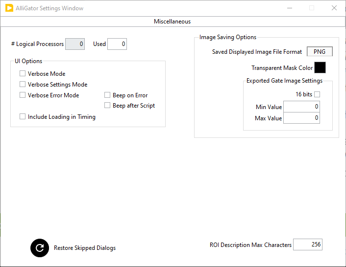
UI Options:
- # Logical Processors Used: select the number of logical processors available to AlliGator for parallel computing. The number of available logical processors is indicated to the left of this control.
- Verbose Mode: if checked off, outputs information on individual processing steps during AlliGator processing (displayed in italics and light gray color in the Notebook). This can be useful to provide a complete record of a workflow.
- Verbose Settings Mode: if checked off, sends a copy of each change in the Settings window to the Notebook (green italics).
- Verbose Error Mode: if checked off, sends a copy of each internal error message to the Notebook (useful for debugging or error reporting purposes). Errors are ignored and do not prevent AliGator from running, but might indicate bugs or incorrect input parameters.
- Beep on Error: if checked off, each error is signaled by a Windows “Critical Stop” sound.
- Beep after Script: if checked off, outputs a Windows “Exclamation” sound.
- Include Loading in Timing: if checked, reports the time spend loading a dataset from file when calculating the time needed to get it into memory.
Image Saving Options:
- Saved Displayed Image File Format: PNG/JPEG/BMP: file format used to save the displayed source image with overlay, the source image overlay, the phasor graph, the phasor plot with overlay or the decay fit parameter map.
- Transparent Mask Color: select the color in the image that will be made transparent in the saved image (works with PNG format only).
- Export Gate Image Settings: conversion settings used to save gate images as 8 or 16 bit images.
  16 bits: if unchecked, exports the image as an 8 bit TIFF file.
  
  Min/Max Value: values used to convert a floating point image to an integer one according to \((I-min)/(max-min)*I_{range}\), where \(I\) is the floating point pixel intensity, and \(I_{range}\) the dynamic range of the destination integer image. If one of the limits (Min or Max) is inf or NaN, the image is clipped to the destination image’s range with the user’s approbation.
- Restore Skipped Dialog: press this button to reset all skippable dialogs so that they show up again.
- ROI Description Max Characters: sets the maximum string length output to the Notebook when exporting a ROI’s description. Warning: the description will be truncated to that length, which will make it impossible to copy and paste it later for reconstruction.