Decay Fit Parameter Map Panel
The Decay Fit Parameter Map panel is used to display and further process multi-ROIs NLSF results (and can be used to display results from a Python plugin if needed).
The panel consists of different controls and indicators as illustrated below and discussed next.
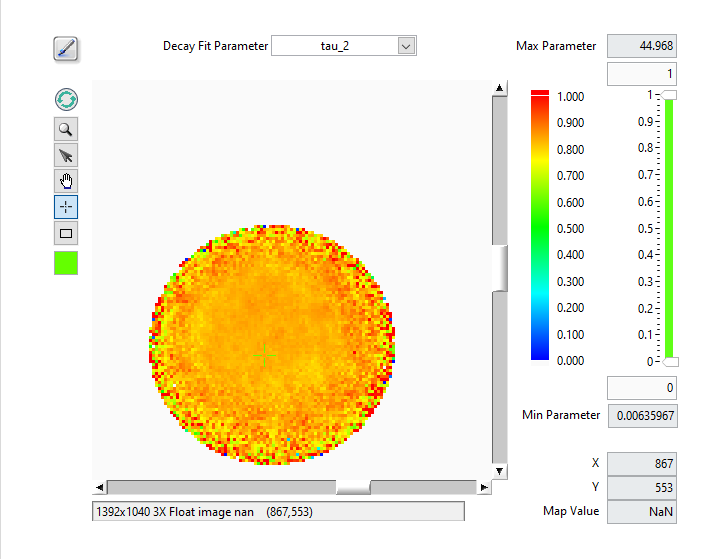
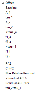
The main object is the map itself, which represents a color-coded image of the selected parameter (Decay Fit Parameter pull-down list at the top right), based on the selected Decay Fit Parameter Map Color Scale (next to the map) and the values of the Decay Fit Parameter Map Display Range (to the right of the color scale).
The Max Parameter and Min Parameter indicators provide the actual total range of the computed parameters, while the controls immediately above and below the slide represent the position of the sliders, which themselves specify what are the selected Min and Max of the displayed parameters.
Any parameter above or below these two limits are color-coded with the unique color boxes located at the top and bottom of the color scale (by default, the bottom color is white, and is therefore not visible in the snapshot above). Left-click above or below the color scale to reveal the color picker window and select the color highlighting parameters respectively above or below the display range minimum).
The X,*Y* and Map Value indicators at the bottom right provide the location of the cursor (also visible in the image information bar below the map), as well as the actual map value at that location. if that latter indicator appears unresponsive, briefly move the mouse out of the window and back to reactuivate mouse tracking (that trick also work to reactivate the Local Decay Graph Window mentioned below).
The square Tools buttons on the top left of the Decay Fit Parameter Map
allow zooming, selecting, moving or clicking the image or a ROI. Note that the
Rectangle tool is only used to zoom in on a specific region of the map in
combination with the Alt key.
The Refresh Parameter Map button forces redrawing the map, while the square color selector at the bottom allows defining the color of the ROIs drawn over the map.
Finally, the Overlay Decay Fit Parameter Map button at the top left (brush tool) enables overlaying the current Decay Fit Parameter Map on the Source Image.
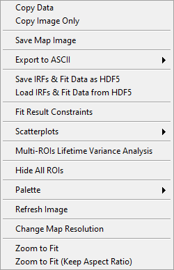
Decay Fit Parameter Map Menu
The Decay Fit Parameter Map context menu is shown below and discussed next.
.
Copy Data: This copies the LabVIEW image object bitmap, including tool palette, scroll bars, and image information.
Copy Image Only: Only copies the visible image.
Save Map Image: Saves the whole image as a PNG file (with dialog).
Export to ASCII:
Export Map Data as ASCII: This will export the current map image as an ASCII matrix of parameter values. If only a few of the image pixels have actual parameters associated with them, this will result in a mostly
NaN-filled file, with a few isolated actual values.Export All Maps Data as ASCII: This will export all parameter map images as separate ASCII matrices of parameter values.
Export ROI Data as ASCII: This function exports all parameters for the selected ROI. Note however that there are 3 different use cases:
If the the ROIs used to compute the map are all single-pixels and the selected ROI is a single-pixel ROI, this will export a single row of parameters, preceded by the ROI index and pixel coordinates.
If the the ROIs used to compute the map are not all single-pixels and the selected ROI is one of the original ROIs used for computing the map, this will export a single row of parameters, preceded by the ROI index and pixel coordinates.
Possibly more interesting, if the the ROIs used to compute the map are all single-pixels but the selected ROI is not, this will export multiple rows of parameters corresponding to the different pixels in that ROI, preceded by the ROI index and pixel coordinates.
Export All ROIs Data as ASCII: Similarly to the previous one, this function exports all parameters for all the ROIs. Again, there are 3 different use cases:
If the the ROIs used to compute the map are all single-pixels and the ROIs are also single-pixel ROIs, this will export multiple rows of parameters, preceded by the ROI index and pixel coordinates.
If the the ROIs used to compute the map are not all single-pixels and the ROIs are the original ROIs used for computing the map, this will export multiple rows of parameters, preceded by the ROI index and pixel coordinates.
Possibly more interesting, if the the ROIs used to compute the map are all single-pixels but the ROIs used are not, this will export multiple rows of parameters corresponding to the different pixels in these ROI, preceded by the ROI index and pixel coordinates.
Save IRFs & Fit Data as HDF5: This saves all the data generated during the fit, as well as the IRFs in a HDF5 file. It is the recommended quick way to save the outcome of an analysis and allows revisiting the results with the help of the next function.
Load IRFs & Fit Data from HDF5: This allows reloading the output of an analysis and work with it (see next) together with the loaded dataset (the dataset is not loaded, neither are the ROIs, which needs to be done separately, if needed).
Fit Result Constraints: opens a windows allowing to specify constraints to obey when computing scatterplots (see next menu item). The Fit Result Constraints window is described in the Fit Result Constraints Window section below.
Scatterplots: submenu to select the type of scatterplot to export to the Lifetime & Other Parameters Graph. These scatterplots can be limited to pixels verifying a set of constraints on fit parameters and derived quantities
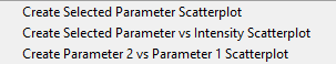
.
Create Selected Parameter Scatterplot: Sends all parameter values P_i in the image as a (i, P_i) scatterplot, where i is the index of the ROI.
Create Selected Parameter vs Intensity Scatterplot: Sends all parameter values P_i in the image as a (I_i, P_i) scatterplot, where I_i is the total ROI decay intensity. This requires the ROIs used during NLSF analysis to be present in order to be able to compute each ROI’s total intensity.
Create Parameter 2 vs Parameter 1 Scatterplot: Opens a dialog window to select the two parameters (P1, P2) to export as pairs.
Multi-ROIs Lifetime Variance Analysis: computes various lifetime variance maps. The results are sent to the Parameter Map panel described in its dedicated page:. See the Lifetime Variance Analysis Maps section for details.
Change Map Resolution: when loading a Decay Fit Parameter Map file, the default size of the map is set to that of the loaded dataset. If that dataset does not correspond to the loaded map data (or no dataset is loaded), it is necessary to manually set the map’s resolution (i.e. image size), which this function allows doing.
The other functions are self-explanatory.
Note that when a series of parameter maps has been calculated, it is possible to visualize the outcome of the fits in a given ROI by opening the Local Decay Graph Window. This will display the local decay, fit, residuals, IRF and residuals autocorrelation function, as well as output the fit parameters and derived quantities in the lower panel of the window.
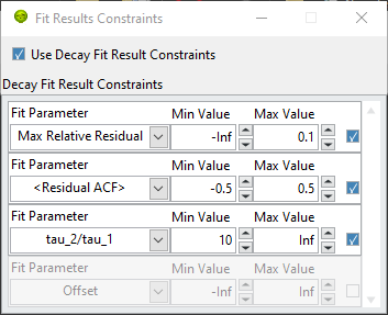
Fit Result Constraints Window
.
The Fit Result Constraints window (opened via the Decay Fit Parameter Map Fit Result Constraints right-click menu item) allows defining Min Value and Max Value for all fit parameters and derived quantities (all quantities available in the Decay Fit Parameter pull-down menu at the top of the panel, plus a few other ones visible in the Fit Parameter pull-down list below).
.
The additional quantities are described next:
Max Relative Residual: maximum of the absolute ratio of the residual over the decay value.
<Residual ACF>: mean value of the residuals autocorrelation function.
Residual ACF SDV: standard deviation of the residuals autocorrelation function.
tau_2/tau_1: ratio of the two lifetimes in a bi-exponential fit (this value is zero for a single-exponential fit).
Note
The ACF is plotted with the zero-point value, but the <Residual ACF> and Residual ACF SDV are computed with this value excluded.
Each constraint line ends with a checkbox indicating whether it should be used or not. Finally, the Use Decay Fit Results Cosntraints checkbox at the top of the list indicates whether or not the selected constraints should be applied. All selected constraints need to be satisfied in order for a pixel to be retained in the analysis.
These constraints may take some time to be computed (especially if max relative residual or residuals ACF are selected), but are only computed once.
Lifetime Variance Analysis Maps
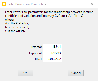
This analysis involves external calibration data establishing the expected lifetime coefficient of variation (\(CV_\tau\)) dependency on intensity (I) for an ideal sample. The analysis requires providing the power law parameters describing this dependency, which are user-provided via the following dialog:
.
The analysis also requires providing parameters defining the intensity slices
to be used in each ROI defined in the image (see the Compute Sliced Mean, SDV
& CV Plots menu of the Lifetime & Other Parameters Panel
for details). This analysis establishes the observed \(CV_\tau(I)\)
dependency.
The following maps are computed:
Delta SDV Map: the map represents the difference between the observed and expected lifetime standard deviation of the selected lifetime map (\(\tau_1, \tau_2, \tau_a\) or \(\tau_i\)), where \(SDV_\tau = CV_\tau*\tau\).
Delta CV Map: the map represents the difference between the observed and expected lifetimecoefficient of variation of the selected lifetime map (\(\tau_1, \tau_2, \tau_a\) or \(\tau_i\)).
Lifetime Variance F-Test Significance Map: the map represents the significance level of the observed lifetime variance ratio using the F-test.
Lifetime Variance \(\chi^2\)-Test Significance Map: the map represents the significance level of the observed lifetime variance ratio using the \(\chi^2\)-test.
(last updated: 2026-01-29)