Local Decay Graph Window
The Local Decay Graph window (opened using the Window:Local Decay Graph
menu item) provides a quick way to explore a loaded dataset at the pixel or
region of interest (ROI) level.
Once the window is opened, use the point or any of the closed ROI tools of the Source Image and click (or draw a ROI) anywhere in the image to display the corresponding intensity decay.
If no NLSF analysis has been performed, this is the only information that is
available. It is similar to using Analysis:FLI Dataset:Current ROI Analysis,
which displays the corresponding decay in the Decay Graph, with the
difference that the display is temporary but adjustable in size (it is still
possible to save the plot to a file or copy/paste it in the Notebook). Think of
it as an exploration tool rather than an analysis tool.
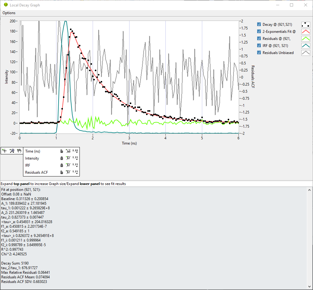
If a NLSF analysis of the dataset has been performed (or a previous analysis has been loaded in the Decay Fit Parameter Map panel), it is not only possible to click in the Source Image, but in the Decay Fit Parameter Map panel as well. Additional curves are plotted, as illustrated in the example below.
.
In that example, the decay is represented as black dots, the fitted model in red, the residuals in green and the IRF in blue. The IRF in this example is local. Finally, the normalized unbiased residuals autocorrelation function (ACF) is represented in grey. The 0-value of the ACF, always large as it is equal to:
is not represented. Note that decay, fit and residuals are associated with the Intensity scale (left), while the IRF is linked to its own vertical scale (not displayed), in order to account for different signal intensities for decay and IRF.
The residuals autocorrelation function is linked to its own vertical scale (shown on the right). A “good” normalized unbiased residuals ACF should indeed have an amplitude of the order of a few units range, which is generally much smaller than most (“good”) recorded decays.
It is recommmended to set the Intensity and IRF scales to autoscale, while the Residuals ACF scale is best set to a fixed range (e.g. [-2, +2] as shown in the example) in order to easily detect when an ACF is problematic.
Decay Fit Information
The lower part of the panel can be independently expanded (or collapsed if not needed) to reveal the stored fit results for the ROI under study. In addition to the fitted parameters and \(\chi^2\) and \(R^2\), the following derived quantities are reported (the last 4 can be used as constraints in Decay Fit Parameter Map analyses):
Decay Sum: Sum of all gate values in the decay.
tau_2/tau_1: Ratio of both lifetimes (in case of a 2-Exp fit).
Max Relative Residuals: Ratio of the max absolute residual value and max absolute decay value.
Residuals ACF Mean: Average of the ACF (not including the 0-value).
Residuals ACF SDV: Standard deviation of the ACF (not including the 0-value).