Image Profile

Any of the open contour tool in the Source Image can be used to look at the image intensity profile and additional information along that contour. Additionally, the Rectangle and Rotated Rectangle tools can be used to analyze averaged profile as discussed in the Averaged Profile section below.

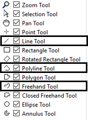
The open contour tools are framed in black in the snapshot below:

For example, using a Line tool on the following image:

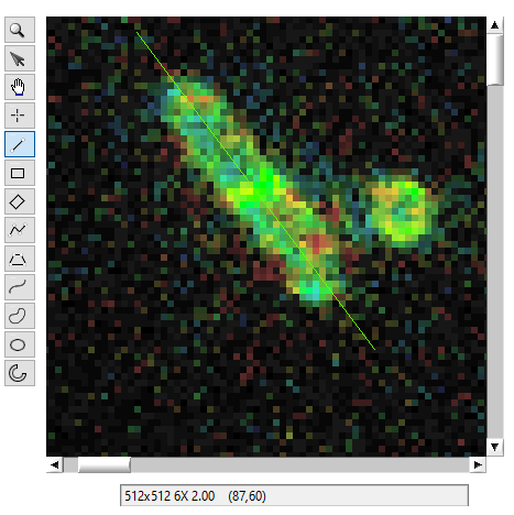
and opening the Image Profile window (Window:Image Profile) results in the following intensity profiles:

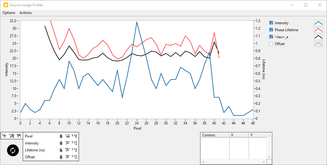
Notice that this graph has two visible vertical scales (Intensity on the left and Lifetime (ns) on the right). In fact, the Scale Legend at the bottom shows an additional (hidden) Offset scale. This scale is used to display one of available decay fit parameters available in the corresponding AlliGator tab. Since no NLSF analysis was performed on this dataset, there is no fit parameter to display and the scale (as well as the plot) was hidden.

The Image Profile window shows the values of other parameters along the contour, provided these parameters are available:

• Intensity

• Phase Lifetime

• Phasor (Intemsity/Amplitude) Ratio/(Intensity/Amplitude)-Averaged Lifetime

• Decay Fit Parameter

If these parameters are not available (for instance because no phasor plot has been calculated, or because no phasor ratio references have been defined, or no decay fit parameter map has been computed), their value will appear as zero.

The decay fit parameter shown last in the Plot Legend is that defined in the Decay Fit Parameter Map Panel. Changing it there will update the corresponding profile plot in the Image Profile graph.

The Image Profile graph is updated each time the contour is modified in the image. For instance, it is possible to grab one end of the line shown at the top and observe the corresponding live update of the graph.

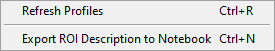
It can also be refreshed using the Actions:Refresh Profiles (Ctrl+R) menu item. Finally, it is updated when one of the display options is modified in the Options menu of the Image Profile window.

The Intensity shown in the graph corresponds to the image selected in the Source Image. In particular, if Single Gate is selected as the Displayed Image, the intensity aling the contour in that single gate will be represented.

Two alternative options accessible via the Options:Image Intensity menu of the Image Profile window are available:

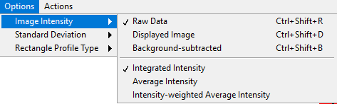
The last three options are only active when using a closed rectangle contour and are discussed later in this section.

In general, the Raw Data’s intensity is represented, but it is also possible to select the Displayed Image option in case the displayed image has been clipped due the location of the Min and Max cursors in the Image Histogram in the corresponding AlliGator panel.

The Background-subtracted option displays the raw intensity minus G x Constant Background per Gate, where G is the number of gates (or bins) in the FLI Dataset and Constant Background per Gate is defined in the Settings:Fluorescence Decay:Decay Pre-Processing panel.

Averaged Profile

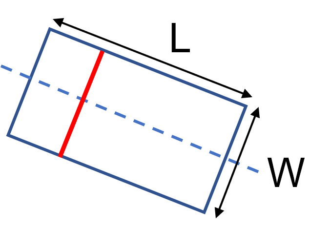
It is possible to average these different quantities using a rectangle or rotated rectangle instead of an open contour. The following schematics explains how this works:

.

The computed profile will contain L values, which will each represent the average along a perpendicular segment of length W (1-pixel wide). The only exception is the intensity profile, which will represent the sum of the pixels’ intensities along the perpendicular segment. Note that the profile will always be measureed along the longest axis of the rectangle. The direction of the profile can be inferred from the label of the Profile Graph.

As usual, if a pixel has been rejected from analysis, it will be excluded from this averaging. If all pixels along a segment are rejected, that average is not computed and replaced by NaN, which does not appear in the displayed profile.

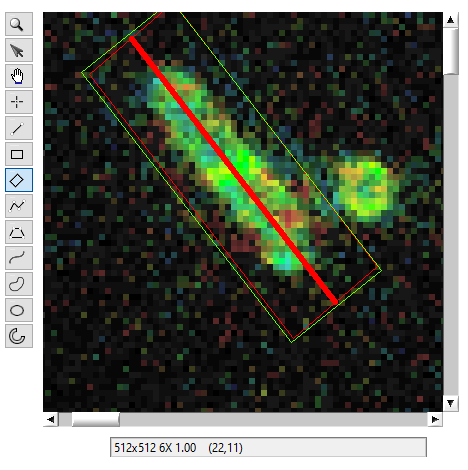
An example is shown below:

.

Notice the green and red rectangles and the thick green center line. The green (sometimes bizzarely deformed) rectangle is the one drawn by LabVIEW. The red rectangle is that overlayed by AlliGator to provide the actual ROI used in the analysis. To show it, check off the Overlay ROI Median checkbox in the Settings:Source Image:Omage Cosmetics window panel. The color of that overlayed rectangle (and the associated center line) is the set by the Median ROI Color box in the same Settings panel.

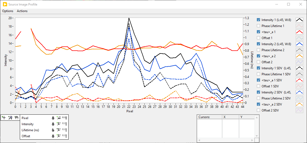
The corresponding Source Image Profile window is shown below:

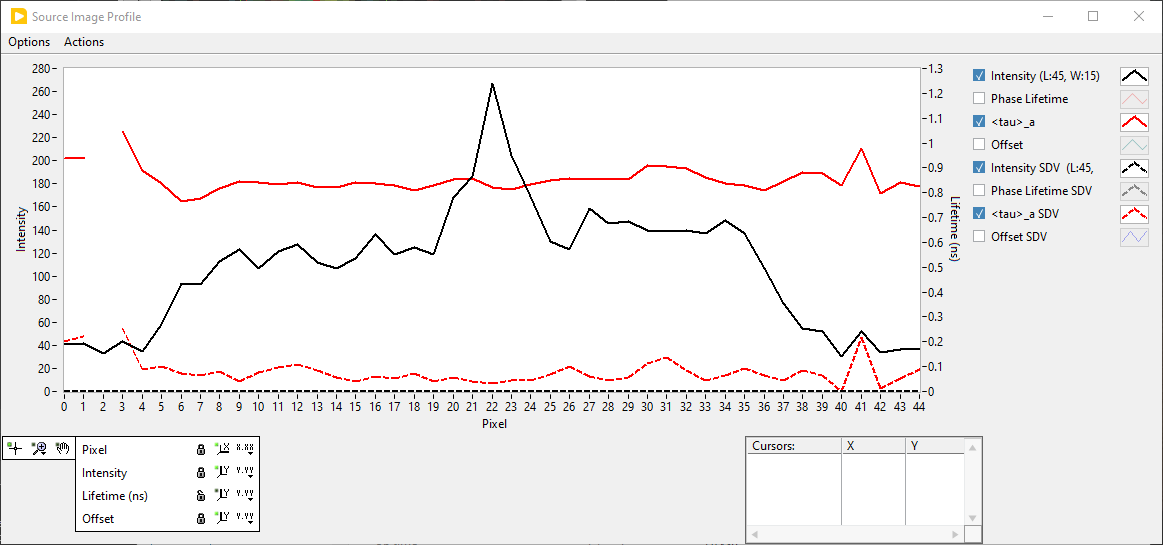
The Phase Lifetime and Offset plots have been hidden, leaving the Intensity and <tau>_a plots, as well as the Intensity SDV and <tau>_a SDV plot (dashed line). The <tau>_a SDV standard deviation plot shown here is the Intensity-weighted one, one of two possible choices:

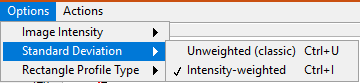
The recommended option is the second one, which calculated the SDV of a quantity f along each perpendicular segment (containing W pixels) according to:

\[SDV = \left( \frac{\sum_{i=i}^{W} I_i f_i^2}{\sum_{i=i}^{W} I_i} - \left(\frac{\sum_{i=i}^{W} I_i f_i}{\sum_{i=i}^{W} I_i}\right)^2\right)^{1/2}\]

This gives less weight to pixels with low intensity, providing a more realistic estimate of the dispersion of the quantity of interest for the brightest pixels.

The classic SDV uses the stadard formula, and will generally be larger, as it could mix background pixels (with a different lifetime) with pixels of interest.

Average Intensity Profile

The intensity data is treated differently than the other quantities, in the sense that in addition to the standard average and intensity-weighted average, the Integrated Intensity" can be represented instead. These options can be selected in the ``Option:Image Intensity menu shown above:

• Integrated Intensity: shows the sum of pixel intensities along the perpendicular segment (red segment in the schematic above). In that case, the calculated SDV is zero.

• Average Intensity: the standard average and dSDV are represented.

• Intensity-weighted Average Intensity: the formula above is used with \(f_i = I_i\).

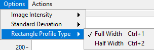
Split Profile

When using a rectangle ROI, it is possible to divide each perpendicular segment into two equal parts and display the average quantity for each of the two halves in the Image Profile graph, by selecting the Option:Rectange Profile Type:Half Width option (Ctrl+2).

Using the example shown above, the resulting split profiles look as shown here:

Current ROI Definition

In order to keep a record of the ROI whose profile is being displayed, it is possible to export its definition to the Notebook using the Actions:Export ROI Description to Notebook (Vtrl+N)menu item: