Fit Method Benchmark
The Fit Method Benchmark window can be opened using the Analysis:Tools:Fit
Method Benchmark menu item. This tool allows computing the effect on fitted
decay parameters uncertainty of a finite signal (total number of collected
photons) using simulations.
The window is comprised of one menu bar and 4 panels, accessible via a drop-down menu located below the menu bar.
Panels
Simulations
Decay, Fit & Residuals Plots
Settings
Script
Each panel is described in the following sections.
Simulations panel
The first panel is where the main parameters of the simulation are defined and the simulation’s results are displayed.
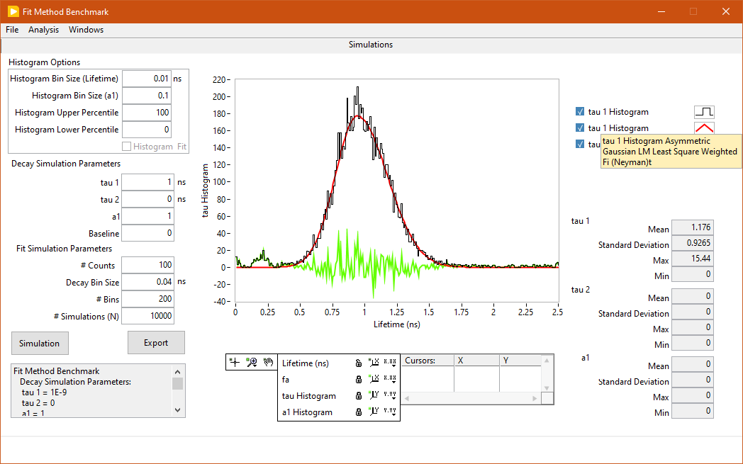
The top four controls on the left are used to adjust the histograms in the center graph, which summarize the simulation’s outcomes.
The next four (Decay Simulation Parameters) specify what kind of decay to simulate (single or double exponential, baseline or none).
Finally, the Fit Simulation Parameters control how many photons per decay (# Counts) need to be simulated, how these photons are binned into a decay (Decay Bin Size and # Bins), and how many times to repeat the simulation (# Simulations (N)). It is important to make sure that the product Decay Bin Size x # Bins remains smaller than the laser period (defined in the Settings panel, Period parameter).
The Simulation button starts the simulation, whose progress is shown with a progress bar at the bottom. Upon completion, one or more histograms are displayed, together with some summary statistics for one of the three possible parameters (1 for single exponential decays, 3 for bi-exponential decays).
This information is also available as text in the Simulation Summary text box below the Simulation button, and is exported to the AlliGator Notebook.
The full parameter output of the N simulations can be exported as an ASCII file by clicking on the Export button. This will create a file with one header line followed by N rows, each containing the following information:
Offset, Offset SDV, Baseline, Baseline SDV, A_1, A_1 SDV, tau_1, tau_1 SDV, R2, Chi2
Note that, in the presence of an asymmetric histogram or an histogram with significant outliers, the summary statistics might be significantly biased. In these cases, it might be preferable to fit the histogram with an appropriate model and extract the relevant metrics from the fit parameters (e.g. Gaussian or Asymmetric Gaussian fit).
Returning to the top left control parameters, they can be used to improve the appearance of the histograms generated after a simulation (they are ineffective on previous histograms):
Histogram Bin Size (Lifetime): use this parameter to adjust the granularity of the lifetime histogram(s). There is only one histogram when the decay is mono-exponential, but two lifetime histograms (tau 1 and tau 2) when it is bi-exponential.
Histogram Bin Size (f1): use this parameter to adjust the granularity of the fraction f1 histogram.
Histogram Lower/Upper Percentile: use these parameters to adjust the range of parameter values retained to build each histogram. Histograms can have no more than 10^5 bins. When a parameter is highly dispersed (with very large or very small outliers), choosing to small a bin size can result in an overflow. No histogram is actually displayed and an error output in AlliGator’s Notebook. To alleviate this problem, either change the bin size or eliminate ouliers by gradually reducing the Histogram Upper Percentile (the Lower Percentile is generally left equal to zero).
Note that the graph has 4 scales: Lifetime (ns), tau Histogram, on one hand
and f1, f1 Histogram, on the other. To show or hide one of the scales listed
below the graph, left-click on the X.XX or Y.YY button in the Scale
Legend and select Visible Scale.
As mentioned above, each histogram can be fitted by one of the many models available via the right-click Fit menu in the plot legend.
Decay, Fit & Residuals Plots Panel
The second panel is used to display the simulated decays, their fits and the corresponding residuals.
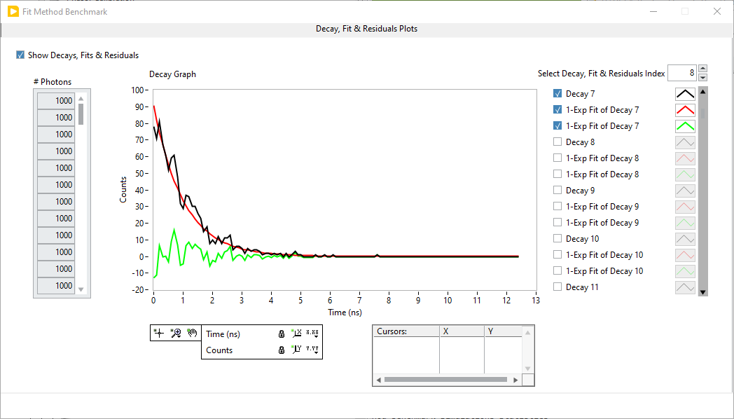
For a number of simulations N > 1000, this can require some additional memory resources. It is therefore recommended to use this display option (active when the Show Decays, Fits & Residuals checkbox is checked off) only as a way to verify that simulations and fits work as expected, using a small N (e.g. N = 100). By default, none of the plots are visible, but they can all be shown using the graph’s right-click shortcut menu.
Alternatively, it is possible to scroll through one decay and its fit and residuals plots at a time using the Select Decay, Fit & Residuals Index control above the plot legend.
This panel is also used to load and visualize the IRF, if an IRF is used in the
simulations (see the Settings Panel description below). To load an IRF, use
the Load Experimental IRF right-click menu item. If an IRF is loaded, it can
be visualized in the Decay Graph by using the Show Experimental IRF
right-click menu item.
Note
The IRF should cover the duration of the laser period, defined in the Settings panel (Period parameter).
Settings Panel
The next panel is used to define fit options and is similar to the corresponding AlliGator Settings panel (Settings:Fluorescence Decay:Fit Options), with some elements of the Settings:Fluorescence Decay:Fit Parameters panel.
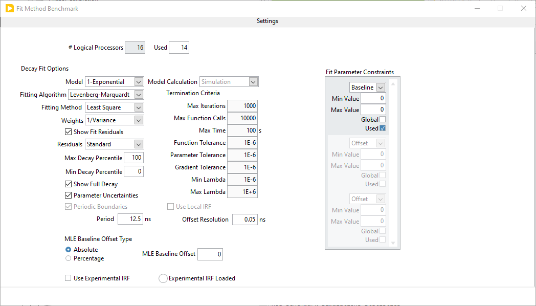
The new elements are:
# Logical Processors Used: define the number of cores to be used for simulations
MLE Baseline Offset Type: the two options are
AbsoluteandPercentage. In the first case, the MLE Baseline Offset parameter is used to add a constant baseline offset to the data before the fit, that constant being subtracted from the fitted baseline after the fit (see discussion below). In the second case, the added baseline offset is defined as a percentage of the decay peak value.Use Experimental IRF: if an experimental (or theoretical!) IRF has been loaded, it will be used to convolve the simulated decays prior to the fitting step (and the IRF will be used during fitting). It is recommended to use the same decay bin size for the simulation as for the IRF. If no IRF is available, this setting is ignored.Experimental IRF loaded: this LED will turn on whenever an IRF has been loaded (see Decay, Fit & Residuals Plots Panel section above).
Note
The MLE Baseline Offset parameter is useful to avoid failure of the Levenberg-Marquardt algorithm when the actual baseline of the decay is small. Indeed, in that case, the fitted baseline might end up negative, which would result in negative fitted values, which are incompatible with the MLE assumption that values are positive (as photon count values). To avoid this, one can introduce an artificial offset enforcing a positive baseline. This temporary offset is subtracted from the fitted parameter before the results are returned.
Scripts Panel
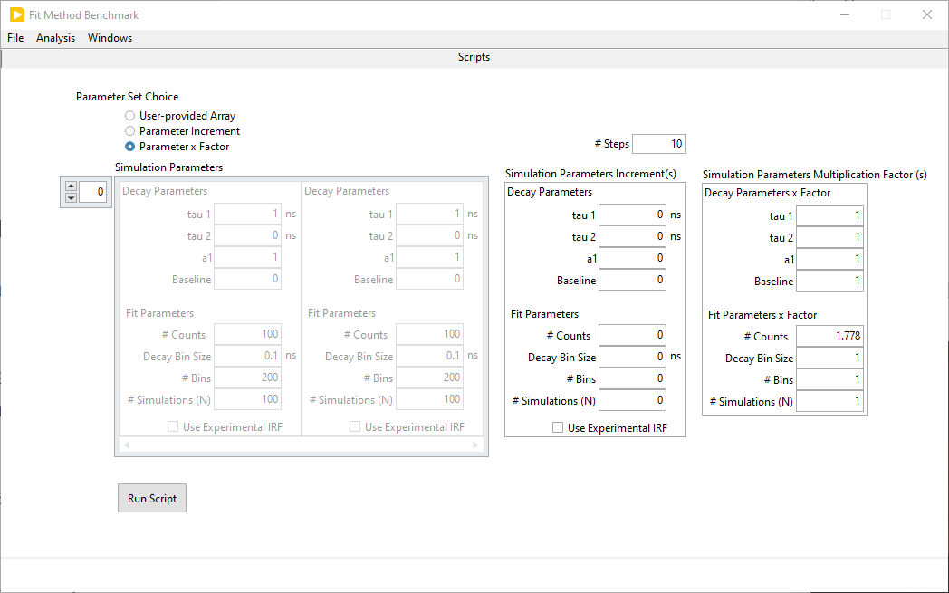
This panel allows defining sets of simulations run sequentially in 3 different ways:
Using a user-provided array of simulation parameters,
Incrementing one or more of the currently defined simulation parameters in the Simulations panel,
Multiplying one or more of the currently defined simulation parameters in the Simulations panel.
The desired approach is selected using the Parameter Set Choice radio buttons at the top left. Next, the parameter sets, or parameter increment(s), or parameter multiplication factor(s), are defined in their respective controls:
Simulation Parameters: enter as many parameter sets as desired. Use the array index control on the top left or the scrollbar at the bottom to define new sets.
Simulation Parameters Increment(s): By default, the increment of all parameters is zero. To increment one or more parameter(s) at each step of the script, change the decay and/or fit parameters to the desired increment value. The first set of Decay Parameters and Fit Parameters used during the script correspond to those defined in the s panel (without the increment(s) applied). Finally, define the # Steps to be used in the script.
For instance, to study the fit method performance for lifetimes in the range 0.5 to 5 ns every 0.5 ns, use a Simulation Parameters Increment(s) tau 1 value of 0.5 ns, leaving all other values = 0, and set # Steps = 10.
Simulation Parameters Multiplication Factor(s): By default, the multiplication factor of all parameters is one. To multiply one or more parameter(s) at each step of the script, change the decay and/or fit parameters to the desired multiplication factor. The first set of Decay Parameters and Fit Parameters used during the script correspond to those defined in the Simulations panel (without the multiplication factor(s) applied). Finally, define the # Steps to be used in the script.
For instance, to study the effect of the number N of photons on the fit method performance for N = 100 to 10,000 using a logarithmic spacing with 4 values per decade, use a Simulation Parameters Multiplication Factor(s) # value of \(10^{1/4} = 1.778\) leaving all other values = 1, and set # Steps = 10.
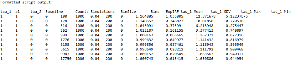
Once defined, the script can be started using the Run Script button or using
the Analysis:Run Script menu item. The output will be # Steps tau 1
histograms (in the case of 1-Exp fits) in the Simulations panel, and a table
of Decay & Simulation Parameters as well as parameter histogram(s) summary
statistics in the Notebook, an example of which is provided below:
The results can also be exported in an ASCII file using the File:Export
Results menu item.