Fluorescence Decay Fitting
AlliGator offers basic capabilities to analyze data using standard techniques of fluorescence decay fitting:
Individual decays can be fitted with a single or double-exponential decay model convolved with or without an experimental instrument response function (IRF).
Multiple ROIs in the image source can be fitted, the resulting parameters being output as maps (see Decay Fit Parameters Map Panel)
Series analysis of a ROI in the image source can be done one ROI at a time (the same ROI is used throughout the series), or a list of ROIs can be used, in dataset in the series using one of the ROI in the list (in the order they appear in the list). In both cases, selected parameters are output as individual plots (one plot per parameter, one point per dataset).
These different capabilities are described next.
Single decay fit
Overview
A single plot can be fitted by a model function convolved with the selected IRF
by right-clicking on its legend (or close to it in the graph) and selecting
Fit Decay. The options specifying the type of fit and the constraints used
are defined in the Settings:Fluorescence Decay:Fit Options and
Settings:Fluorescence Decay:Fit Parameters panels respectively.
Several fit options, discussed below, are available in the Settings:Fluorescence Decay:Fit Options panel:
Model
Fitting Algorithm
Fitting Method
Weights
Show Fit Residuals
Residuals
Max & Min Decay Percentile
Show Full Decay
Parameter Uncertainties
Periodic Boundaries
Period
Use Data Information Laser Period
Termination Criteria
Use Local IRF
Offset Resolution
Parameter constraints, guess parameters and whether or not to display the output as plots are managed in the Settings:Fluorescence Decay:Fit Parameters panel
Fit with constraints applied on individual parameters is handled by an array of Fit Parameter Constraints specifying the:
Parameter
Min & Max Value
whether or not it is a Global parameter (applicable in case of multiple fits only)
whether the constraint is used or not
Guess parameters can be provided in the corresponding array by selecting the parameter name and providing the guess value. Additionally, the way these parameter guesses are used (or not) can be dedined via the Options pull-down list:
Numerically Estimated
User-provided
User-provided (normalized)
Last valid fitted parameters
The Displayed Fit Parameters array only applies to series analysis and will be discussed in that context in a later section.
Fit Options
Model: Two models are currently available.
A single exponential (1-Exponential) model defined by:
\(f\left( t \right) = {A_1}\exp \left( { - \frac{t}{{{\tau _1}}}} \right) + b\)
where b is the baseline and the IRF is offset by an amount (i.e. centered at) \(t_0\).
A double exponential (2-Exponentials) model defined by:
\(f\left( t \right) = {A_1}\exp \left( { - \frac{t}{{{\tau _1}}}} \right) + {A_2}\exp \left( { - \frac{t}{{{\tau _2}}}} \right) + b\)
Fitting Algorithm: currently, the Levenberg-Marquardt algorithm in the only one implemented.
Fitting Method: 4 methods are available:
Least Square
Least Absolute Residuals
Bisquare
MLE
Weights: Two types of fits can be performed:
Unweightedfit where all data points are equally weighted in the minimization function (sum of difference squared)1/Variance, where each data point i is weighted by \(1/{f_i}\) (or 1 if \(f_i = 0\)), where \(f_i\) is the function value.
Residuals: The fit residuals (difference between the original decay and its fit) can be optionally plotted in addition to the fit itself. Several options can be chosen:
The standard residual is the mere difference between the original decay and its fit, while the normalized residual is the difference divided by the function value. The reduced residual is the difference divided by the square root of the absolute value of the function value.
Min & Max Decay Percentile: The fit can be performed over the whole decay or limited to the “tail” part of the decay. The latter is defined as the part of the decay located between XX% of the decay maximum (max percentile) and YY% (\(0 \le YY < XX \le 100\)) of the decay maximum (min percentile).
Show Full Decay: When only part of the decay is fitted, it is possible to show the fitted curve (and residuals, optionally) calculated over the full decay range by checking this checkbox. The default (unchecked) is to only show the decay over the selected range.
Parameter Uncertainties: Because parameter uncertainty calculation involves computing the covariance matrix of all parameters, this can be very memory consuming in the case of global fit of large data sets. In that case, it might be desirable to skip calculation of parameter uncertainties by leaving this checkbox unchecked.
Periodic Boundaries: This option enforces periodic boundary conditions. The laser repetition period can be entered in the Period box below or the Use Data Information Laser Period can be checked.
This is mostly useful for large gates (e.g. SwissSPAD data) for which the resulting decay does not look anymore as a sharp rise followed by a tail decaying to background level, but instead as a continuous “wave”. In these conditions, it is advantageous to treat the decay as periodic. Note that the recorded decay needs to be no longer than the provided period for the fit to be any good (it can be shorter, i.e. truncated).
Model Calculation: Currently only a Convolution approach is available. It is based on FFT and works best with an IRF covering the whole laser period.
Termination Criteria: These parameters provide some control on the way convergence of the Levenberg-Marquardt (LM) algorithm is aasessed.
Max Iterations: This controls the number of iterations of the LM algorithm to perform before stopping optimizing the cost function for a given offset parameter.
Max Function Calls: controls the number of calls to the code computing the model values and/or its derivatives. This number is generally close to twice the previous one.
Max Time: sets the maximum time spent iterating the LM algorithm.
Function Tolerance: Minimum relative change in cost function to achieve in order to stop the LM algorithm.
Parameter Tolerance: Minimum relative change in any of the model parameters to stop the LM algorithm.
Gradient Tolerance: Minimum relative change in the RMS of the models function’s gradient.
Min & Max Lambda: Min & Max value of the LM algorithm’s scale parameter.
Use Local IRF: When a set of local IRFs has been defined, instructs the software to use it (rather than a common IRF defined by the user in the Decay Graph)
Offset Resolution: The (IRF time) offset parameter is treated separately from the other model parameters. All values in the specified constraint range are tried by stepping through in increment of Offset Resolution, in order to obtain the value for which the fit of the other parameters results in the minimal value for the cost function. A small value of this parameter may increase the precision of that parameter but will result in a longer fit duration.
Fit Parameters
Fit Parameter Constraints: Fit parameters can be constrained within a specified range defined by the min (-Inf if unconstrained) and max value (Inf if unconstrained).
The list of actual parameters that can be constrained depends on the chosen model:
For instance, choosing \(tau_2\) as a constrained parameter in a 1-Exponential model will have no effect.
If a parameter is unconstrained, it is possible to remove it from the array of
constrained parameters by right-clicking on it and choosing Delete Element.
If no parameter is constrained, it is possible to delete all elements of the
array by right-clicking on the scrollbar and choosing Empty Array.
Alternatively, checking off the Used checkbox will ignore this constraint.
Guess Parameters: Convergence of the LM algorithm can sometimes be sped up by providing guesses for one or more parameters of the model. Note that bad guesses can also throw the algorithm off track and prevent obtaining a good fit. Regardless, the algorithm requires starting values for all parameters. There are a few options to provide those:
Numerically estimated: simple guesses based on the decay curve are computed for all parameters
User-provided: user-provided values are used for parameters that have them, numerically estimated ones for the others.
User-provided (noemalized): parameters are provided for the normalized decay (for which the maximum value is 1). This allows providing relative amplitude values rather than absolute ones.
Last valid fitted parameters: uses the last successful fit parameters.
Displayed Fit Parameters: When performing a Series fit, this array determines which fit parameters are output as a plot in the Lifetime & Other Parameters graph. Leave the arra empty for all parameters to be output.
Fit Results
In addition to the plot output(s) in case of a successful fit, the fit results are output to the Notebook. A typical output will read:
2-Exponentials weighted fit of XXXXX

Model Calculation: Convolution
Use Local IRF: FALSE

Periodic with  (SYNC) period: 12.5 ns
CPU: 0.120509 s
Fit range: 0%-100%
Fitting Algorithm: Levenberg-Marquardt
Fitting Methods: Least Square
Total number of iterations: 201
Max number of iteration per offset value: 201 [<200]
Total number of function calls: 202
Max number of function calls per offset value: 202 [<1000]
Gradient: 3.828665E-5 [1E-6]
|Delta Chi2|: 3.138666E-7
|Delta Chi2|/Chi2: 0.000428 [1E-6]
Max |Delta a/a|: 0.017266 [1E-6]
Lambda: 0.012433 [1E-6, 1000000]
Termination criterion: Max Iterations Exceeded
Residual Sum of Squares (RSS): 0.060079
Akaike Information Criterion (AIC): 397.180562
Bayesian Information Criterion (BIC): 474.215033
Guess Fit Parameters:
Type: Numerically estimated
Offset: 0
Baseline: 0.001465
A1: 0.445958
tau 1: 0.865617
A2: 0.445958
tau 2: 2.596851

Fitted Parameters:
Offset: 0 ± NaN [0, 0]
Baseline: -0.03914 ± 0.004655 ]-Inf, +Inf[
A1: 2.828889 ± 0.990132 [0, Inf]
tau 1: 0.676268 ± 0.117808 [0, Inf]
A2: 0.698186 ± 1.025203 [0, Inf]
tau 2: 1.326534 ± 0.578591 [0, Inf]
Amplitude-averaged lifetime: 0.80498
Intensity-averaged lifetime: 0.888374
R^2: 0.997084
Chi^2: 0.500797
Reduced Chi^2: 0.002555
Standard residuals
Plot(s) added to Decay Graph: 2-Exp Fit of XXXXX, 2-Exp Fit of XXXXX Residuals
where XXXXX is the decay name. \(R^2\) and the reduced \(\chi ^2\) as well as the 68% confidence intervals (errors) are defined according to the definitions provided here If the fit fails, an error message will be displayed instead (and not plot added to the Decay Graph).
Series decay fit
In the case of a series analysis, decay fits can be performed by choosing
FLI Dataset Series:Series NLSF Analysis:Current ROI or :Sequential ROIs``
in the Analysis menu.
Each time point decay is fitted separately, following the protocol described previously for single decays. In addition, it is possible to generate one or more plots of the evolution of selected fit parameters across the series, using the Displayed Fit Parameters array. These plots will be output in the Lifetime Graph of the Lifetime Analysis panel (see corresponding manual page). Parameters that can be displayed can be chosen from the following list:
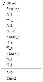
This list includes the fit parameters and derived quantities, such as the mean lifetimes <tau>_a and <tau>_i or fractions f1_a and f1_i (for the 2-Exponentials model, defined below), or the \(R^2\) and \(\chi ^2\) outputs.
amplitude-averaged lifetime |
intensity-averaged lifetime |
|---|---|
\(\left\langle \tau \right\rangle_a = f_{1a}\tau _1 + f_{2a}\tau _2\) |
\(\left\langle \tau \right\rangle_i = f_{1i}\tau _1 + f_{2i}\tau _2\) |
\(f_{1a} = \frac{A_1}{A_1 + A_2}\) |
\(f_{1i} = \frac{{{A_1}{\tau _1}}}{{{A_1}{\tau_1} + {A_2}{\tau_2}}}\) |
\(f_{2a} = 1 - f_{1a}\) |
\(f_{2i} = 1 - f_{1i}\) |
Note that the above definitions are only valid in the approximation of large laser period (compared to the respective lifetimes). The exact formulas are:
amplitude-averaged lifetime |
intensity-averaged lifetime |
|---|---|
\(\left\langle \tau \right\rangle_a = f_{1a}\tau _1 + f_{2a}\tau _2\) |
\(\left\langle \tau \right\rangle_i = f_{1i}\tau _1 + f_{2i}\tau _2\) |
\(f_{1a} = \frac{A'_1}{A'_1 + A'_2}\) |
\(f_{1i} = \frac{{{A'_1}{\tau _1}}}{{{A'_1}{\tau_1} + {A'_2}{\tau_2}}}\) |
\(A'_i = A_i \left(1 - \exp{(-T/\tau_i)} \right)\), i = 1 or 2 |
\(A'_i = A_i \left(1 - \exp{(-T/\tau_i)} \right)\), i = 1 or 2 |
\(f_{2a} = 1 - f_{1a}\) |
\(f_{2i} = 1 - f_{1i}\) |