Decay (Pre-) Processing

A number of operations and processing options can be applied to ROI decays, either as they are extracted from a dataset (in that case, the decay is “pre-processed”), or after they have been displayed in the Decay Graph (in which case, the decay is merely “processed”).

Available operations and associated options are defined in the Fluorescence Decay:Decay Pre-Processing panel of the Settings window.

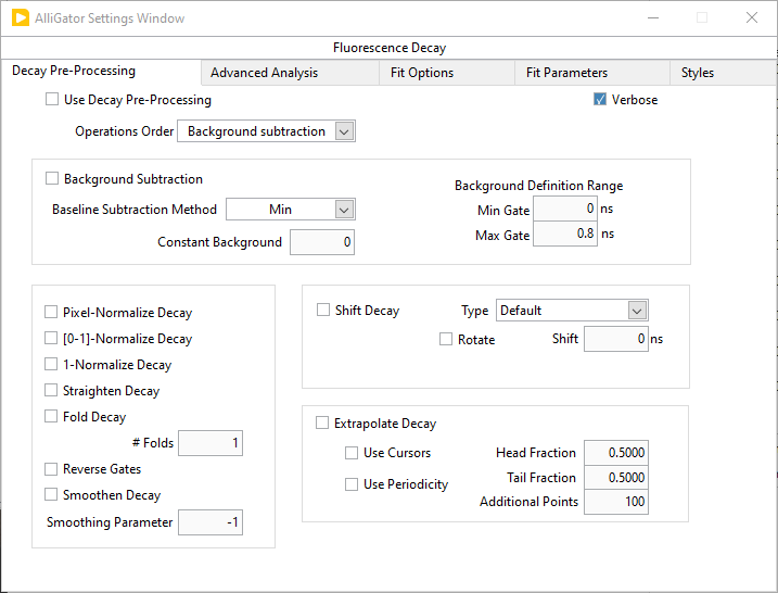
These options are applied to newly computed decays only if the top left Use Decay Pre-Processing checkbox is checked. These pre-processing operations can also be applied one at a time to existing decays using the right-click menu (Process Plot(s)) in the Decay Graph. In that case, the Use Decay Pre-Processing checkbox does not need to be checked.

The order of the decay pre-processing operations applied to newly computed decays is user-selectable. For instance, in the case of photobleaching or photobrightening, this allows correcting for that effect before attempting a square-gated single-exponential background subtraction is applied.

To change the order of operations, right-click on the Operations Order list and select Reorder Operations: this will open a window showing the current list order:

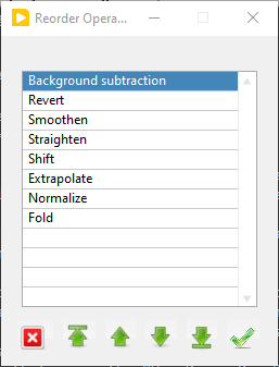
Selecting any of the items, use the buttons at the bottom to change the order of that item in the list. When done, click the OK button (rightmost button) to accept and close the window, or the Cancel button (leftmost button) to cancel any modifications to the original list. Closing the window is equivalent to cancelling and accepting that choice.

The following is a description of the different operations in the order they appear in the Settings:Fluorescence Decay:Decay Pre-Processing panel.

Background Subtraction

There are 4 different methods (not including background file subtraction) to define the value to subtract from each decay point. They are listed in the Baseline Subtraction Method pull-down list as: Mean, Min, Square Gated Single Explonential and Constant.

1. Mean or Min Baseline

It is customary in time-gated imaging experiments to offset the decay on the time axis in such a way that a flat (background) zone precedes the actual rise and decay. This trailing” part of the decay can therefore be used to estimate the background for each ROI (and by extension, for each pixel). The user needs to define the Min Gate and Max Gate locations to be used for background estimation. The actual value retained as background is the minimum (Min) or average (Mean) value recorded in this gate interval.

2. Square Gated Single-Exponential method

In this approach (Square Gated Single-Exponential), the recorded decay is assumed to be the result of a single-exponential decay integrated over a square gate of duration W (See description in ref. 2 in the Bibliography page). The user needs to provide the gate positions where the known minimum (Min Gate) and maximum (Max Gate) of the decay are observed (best obtained by looking them up on a reference decay with high SNR). The analysis computes the Baseline value (which will be used for background subtraction), Amplitude and Lifetime associated with the decay and displays them on the top right of the Fluorescence Decay panel. These parameters as well as the total integrated intensity are associated with the decay and the corresponding phasor plot data point (Phasor Graph panel).

3. Constant Background

It is possible to provide a user-specified background value to subtract from decays using the Constant option of the Baseline Subtraction Method and entering the desired background value in the Constant Background control.

Decay Normalization

Decays can be normalized to a maximum value of 1 (by dividing by the maximum value), or mapped to the [0, 1] interval (by subtracting the minimum and dividing by the decay range), by checking the 1-Normalize Decay checkbox or the [0, 1] Normalize Decay one.

Alternatively, the decay can be divided by the number of pixels comprising the source ROI by checking the Pixel Normalize Decay.

Decay Straightening

Occasionally, samples can photobleach (or photobrighten) during the course of a series of gate acquisition. This phenomenon is identifiable by the fact that the recorded gate value at the end of a complete laser period is different (generally smaller but sometimes larger) than at the beginning of the period. The straighten function assumes that this is due to an exponential decay (or increase) of the signal due to some underlying phenomenon, and attempts to calculate the time scale of this variation as well as its amplitude, and finally, correct for it accordingly throughout the gate sequence. Up until version 0.18.1, this correction was applied as follows:

where \(F_{min}\) is the minimum decay value, T is the period, \(\tau\) is the photobleaching/photobrightening time constant obtained from:

The sign of \(\tau\) obtained from the above equation handles both cases. After version 0.18.2, the correction does not consider that the decay consists of a constant background \(F_{min }\) added to a photobleaching/photobrightening component, as this background component should be taken care of by the background subtraction step, which usually precedes (*) all other pre-processing steps. As a consequence, the formula becomes:

where \(\tau\) is given by:

This equation requires that F(0) and F(T) be non-zero and if no photobleaching/photobrightening occured, identical. In other words, the decay needs to be shifted such that the maximum of the decay is the first gate, and the last gate corresponds to the same location in the decay (it will therefore not work with a truncated decay, and in fact will require an extra gate beyond the laser period).

(*) Note that since version 0.19, it is possible to change the order of the different decay pre-processing operations (except pile-up correction, which remains the first operation). This means that if background correction follows decay straightening, the assumption of the straightening algorithm may be incorrect (i.e. the algorithm will assume that both decay and background exponentially increase or decrease with the same time constant).

Decay Folding

Decay folding consists in dividing the decay in an integer number n of equal segments and summing them up to form a decay n times shorter. The segments’ length should obviously be equal to a multiple of the laser period for this to have a physical sense.

Gate Reversing

When selected it, changes the direction of the plotted decay, so that the tail of the decay comes after the rising part.

Decay Smoothing

Occasionally, a decay may be affected by undesirable “spikes”. It is sometimes possible to remove those spikes using cubic basic spline smoothing (details can be found at http://zone.ni.com/reference/en-XX/help/371361P-01/gmath/cubic_spline_fit/). The Cubic Spline Fit implementation of LabVIEW is used without weights, and smoothness parameters identically equal to 1 for all points, and balance parameter equal to 1 -10^(-x), where x is the Smoothing Parameter defined in the Settings:Fluorescence Decay:Decay Pre-Processing panel. From the Cubic Spline Fit description page linked to above:

• If x = 0, the cubic spline fit is equivalent to a linear fit. If x = Inf, the cubic spline fit interpolates between the data points.

• If x < 0, an appropriate value is automatically calculated according to the time axis values.

To use this algorithm as part of the decay pre-processing, check the Smoothen Decay checkbox. The only exposed parameter for this algorithm is Smoothing Parameter. Alternatively, an existing decay can be post-processed (creating a new plot) using the Process Plot(s):Smoothing Decay Graph right-click menu (see below).

Decay Shifting

Decays can occasionally “shift” along the time axis due to several possible causes (in general, setup instabilities). While this is normally not causing problems if data is properly calibrated, it is possible to force alignment of all decays along the time axis by checking the Shift Decay checkbox. There are several options associated with this functionality.

• Type: this drop-down list gives access to 4 modes described below:

• Rotate: this checkbox specifies whether the shift results in a rotation of the decay (considered periodic) or whether to pad the decay with zeros and discard points corresponding to negative abscissa.

• Shift: this parameter has different interpretation depending on the type of shift selected (see below for details) and is not always visible.

• Threshold: this parameter is used in the Threshold mode only (see below for details).

Decay shift types details

• Default: in this case, a constant shift is applied to all decays. This can for instance be useful to align the peak of a given sample to the zero point, or align decays acquired with different setups, etc.

• CFD: the constant fraction discrimination mode applies a constant shift to each decay before inverting it (multiplying it by -1) and adding it to the original decay. The effect of this operation, provided the shift is of the order of the IRF width or smaller, is to create a curve looking like a “chirp”, with a positive bump followed by a negative one, with a zero point in between. This point is generally stable if the shape of the decay is relatively constant (the amplitude can vary). The position of the zero-crossing point is then compared to that of the stored Reference Decay and the difference between these two positions is defined as the decay shift.

• Threshold: in this mode, the provided Threshold parameter is used to find the first location in the decay where this threshold is crossed (from below). This location is compared to that obtained for the store Reference Decay and the difference between these two positions is defined as the decay shift.

• Cross-Correlation: in this mode, the cross-corelation of the decay and the stored Reference Decay is computed and the position of its maximum determined and returned as the decay shift.

At the end of a series of decay analysis, it is possible to plot the calculated shifts in the Lifetime & Other Parameters Graph of the Lifetime & Other Parameters panel, using the Plot Decay Shifts context menu item in that graph.

Decay Extrapolation

In case the decay tail doesn’t reach the background level, the resulting phasor will be offset by an amount that will depend on the final value reached by the decay. It is possible to compensate artificially for this truncation by extrapolating the decay with an exponential tail.

Likewise, if the IRF used for NLSF analysis by decay model reconvolution with the IRF, a truncated IRF may potentially affect the quality of the computed convolution product, which IRF extrapolation may improve upon.

The parameters defining the range of the extrapolation are defined in Settings:Fluorescence Decay:Decay Pre-Processing under the Extrapolate Decay checkbox.

• Use Cursors: this checkbox allows choosing between using cursor locations or fractional values to define the Tail and Head start and end locations. Two cursors need to be created in the Decay Graph using the Process Plot(s):Extrapolation:Create Head & Tail Bounding Cursors menu item. Their locations can be stored in the two Head Fraction and Tail Fraction controls in the Settings:Fluorescence Decay:Decay Pre-processing panel by using the Process Plot(s):Extrapolation:Store Cusor-define Head & Tail Fractions meun item of the Decay Graph.

• Head Fraction: defines what fraction of the decay (starting from the beginning) is used to perform a fit to a single exponential decay. This part of the decay will be shifted to the end (either past the requestd additional points or past the laser period, see below).

• Tail Fraction:specifies what fraction of the decay (starting from the end) is used to perform a fit to a single exponential decay.

• Additional Points parameter specifies how many points (spaced as in the original decay) to add to the decay.

• Use Periodicity: instead of requesting a number of points to be added to the decay, one can ask for enough points to be added to reach the end of laser period by checking this box.

Other Decay Processing Functions

Other decay processing functions are accessible via the Decay Graph context menu. Most of the context menu items are self-explanatory. Items are grouped in different categories of functions:

Edit plot Visibility (and plot style) functions Deletion functions Save functions Load Plot(s) Plot processing Fitting functions IRF-related functions Graph copy/export/visibility functions

As for all graphs in AlliGator, the checkboxes in front of plot names in the graph legend have a dual function. When checked, the plot is visible AND selected. When unchecked, the plot is hidden AND deselected.

Single plot functions can be used by right-clicking on the plot of interest in the graph or its legend. Note that the Export menu is a bit different in this respect: to export a single plot to the clipboard as an ASCII formatted data set, right-click on that plot’s legend (the graphic part of it). To export the WHOLE graph (including hidden plots), right-click in the graph region. Selected plots (or individual plots) can be directly saved in an ASCII file using the Save functions of the above menu.

• Edit Plot

This menu item opens the plot on which the user has right-clicked in the Plot Editor, where several basic operations can be performed.

Warning: the edited plot replaces the original plot unless the Copy button is pressed. It is possible to cancel the operation at any time while in the Plot Editor.

Plot Editor functionalities are described in the corresponding page of the manual.

• Process Plot(s) submenu

  

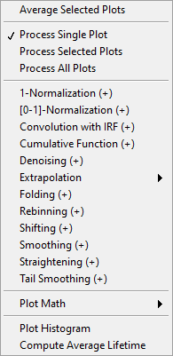
  • Average Selected Plots: This function does what it says and creates an additional plot.

  • Process Single Plot: This option does not do anything on a plot, but is used to instruct AlliGator to operate on a single plot. The checkmark in front of it indicates that this is the current mode of operation for all the functions in the menu followed by the (+) suffix.

  • Process Selected Plot: This option does not do anything on any plot, but is used to instruct AlliGator to operate on all selected plots. The checkmark in front of it indicates that this is the current mode of operation for all the functions in the menu followed by the (+) suffix.

  • Process All Plots: This option does not do anything on any plot, but is used to instruct AlliGator to operate on all plots. The checkmark in front of it indicates that this is the current mode of operation for all the functions in the menu followed by the (+) suffix.

  • 1-Normalization: applies the 1-Normalization operation described in section 2 above.

  • [0-1]-Normaliztion: applies the [0-1]-Normalization operation described in section 2 above.

  • Convolution with IRF: convolves the selected plot(s) with the stored reference decay.

  • Cumulative Function: computes the cumulative function of the selected plot(s).

  • Denoising: processes the selected plot(s) with the Wavelet Analysis Denoise algorithm (see https://www.ni.com/docs/en-US/bundle/labview-advanced-signal-processing-toolkit-api-ref/page/lvwavelettk/wa_de_noise.html for details) using the Wavelength Analysis Options defined in the Settings:Fluorescence Decay:Advanced Analysis panel.

  • Extrapolation:Extrapolate Plot: extrapolates the selected plot(s) as described in section 8 above.

  • Folding: folds the selected plot(s) as described in section 4 above.

  • Rebinning: changes the bin size of the selected plot(s). A dialog window opens up to define the new (larger) bin size.

  • Shifting: shifts the selected plot(s) as described in section 7 above.

  • Smoothing: smoothes the selected plot(s) using cubic splines as described in section 6 above.

  • Straightening: straightens the selected plot(s) as described in section 3 above.

  • Tail Smoothing: smoothes the tail (part of the decay past the maximum) of the selected plot(s) using cubic splines as described in section 6 above.

  • Plot Math: this sub-menu comprises the following functions:

    • y -> f(y) Transform: selecting this item opens up a dialog window to enter an algebraic formula: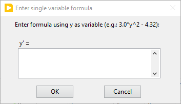

      

    The corresponding amplitude values of the plot (y) will be modified and replaced by y’ as defined by the formula (assuming that the syntax is correct. For a list of supported functions, please refer to this LabVIEW help page).

    • (x, y) >> (f, g)(x, y) Transform: selecting this item opens up a dialog window to enter an algebraic formula: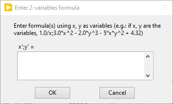

      

      The corresponding time (x) and amplitude (y) values of the plot will be modified and replaced by (x’, y’) as defined by the formulas (assuming that the syntax is correct. For a list of supported functions, please refer to this LabVIEW help page).

    • Two-Plot Algebra: selecting this item opens up a dialog window to enter an algebraic formula: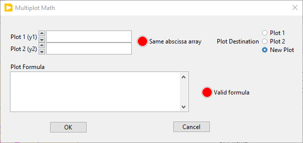

      

      The two plots to be processed can be selected in the Plot 1 and Plot 2 pull-down lists. Only plots with identical abscissa (time axis) can be processed. The Same abcissa array LED turns green when this is the case.

      The first plot is referred to as y1 and the second plot as y2 in the Plot Formula box below, in which the desired formula can be entered.

      Example of valid Plot formula (where y1 represents the value of plot 1 at a given abscissa and y2 the value of the second plot at the same abscissa):

      2*y1 - 3*y2/((1.5e(-3))+y2)

      The list of supported functions can be found at https://www.ni.com/docs/en-US/bundle/labview/page/lvhowto/formula_node_and_express.html

      The list of supported operators can be found at: https://www.ni.com/docs/en-US/bundle/labview/page/lvhowto/precedence_of_operators_in.html

      Note that the exponentiation operator is ‘**’, i.e. the square of y is noted y**2.

    • Plot Histogram: selecting this item opens up a dialog window allowing specifying options to define the way the histogram of the selected decay’s values is computed. The computed histogram is displayed in the separate Histogram Window.

    • Compute Average Lifetime: computes the average lifetime of the selected decay using Average Lifetime Options defined in the Fluorescence Decay:Advanced Analysis panel of the Settings window.